The Properties window is the primary interface in Earth Volumetric Studio for viewing and editing the parameters of various objects within your application. These objects can include modules, output ports, or the application itself. All properties for a selected object are displayed here, organized into logical, collapsible categories.
Module properties:
Application properties:
Port properties:
Accessing the Properties Window
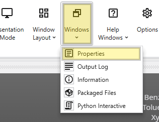
If the Properties window is not already open, navigate to the Windows button in the Main Toolbar to show it.
Editing Objects
Once the window is visible, you can load an object’s properties for editing. The most direct method is to double-click a module or a port of a module in the Application Network. Alternatively, you can use the Choose Object to Edit dropdown menu at the top of the Properties window, which provides a list of all objects in your application and allows you to quickly switch between them.
Navigating and Filtering Properties
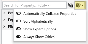
The Properties window includes several tools to help you find and manage parameters efficiently. A Search for Property box at the top of the window allows you to filter the displayed properties by typing a search string; you can also use the Ctrl+P keyboard shortcut to focus on the search box. Next to the search box, the Collapse Categories button lets you expand or collapse all property categories at once.
Options
Further customization is available through the Options menu, accessible via the gear icon. These are global settings for the Properties window and allow you to change how properties are displayed.
Option
Description
Automatically Collapse Properties
When enabled, all property categories are collapsed when properties of a new object are loaded.
Sort Alphabetically
Changes the order of properties to an alphabetical sorting.
Show Expert Options
Reveals advanced parameters.
Always Show Critical
Ensures essential properties are never hidden.
Toggling Module and Display Properties
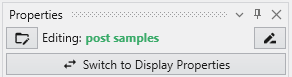
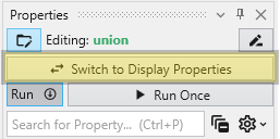
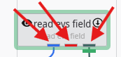
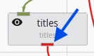
The Switch to Display Properties button allows quick switching between the properties of the selected module and the properties of the primary red output port of it, if it has one. This is the same as double-clicking on the primary red port, but allows faster swapping right within the Properties window.
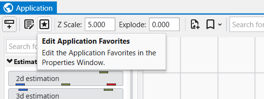
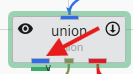
Toggling Application Properties and Application Favorites
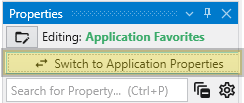
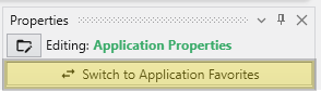
The same button when shown in the Application Properties is labeled Switch To Application Favorites. It allows toggling between the two.
Property Descriptions
At the bottom of the Properties window is a description area. When you select a property from the list, this area displays a brief explanation of what the property does and how to use it, providing helpful context as you configure your modules.
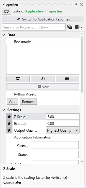
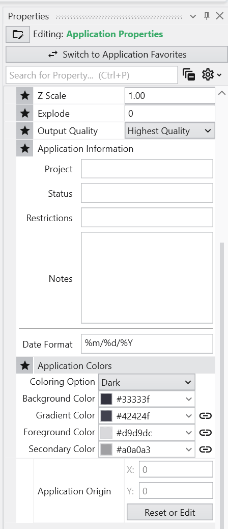
The Application Properties provide a centralized location to access critical parameters needed to control your application. Any property that impacts the application itself and is not specific to an instanced module will show here.
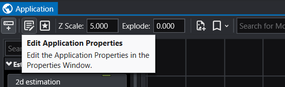
Accessing Application Properties The Application Properties are available via a button in the Application Window toolbar:
Module Properties When you select a module in the Application Network, its settings are displayed in the Properties window. This window allows you to configure the module’s parameters and control its execution behavior. At the top of the window, the name of the module you are editing is displayed.
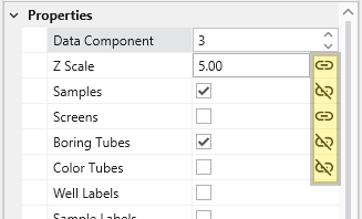
Understanding Linked Properties In Earth Volumetric Studio, a Linked Property is a parameter whose value is automatically determined within the application, rather than being manually set by the user. This dynamic connection allows for a more intelligent and consistent workflow. You can identify a linked property by the link icon located next to it in the Properties window
Port Properties When you double-click an output port on a any module in the Application Network, the Properties window displays detailed information and settings for that specific port. While the properties shown vary depending on the type of data the port provides, certain elements are common to all ports.
Introduction to Datamaps In the fields of scientific and geometric visualization, a datamap is a fundamental concept that serves as the bridge between raw numerical data and its visual representation. At its core, a datamap is a function or a lookup table that translates data values into visual properties, most commonly color. Think of it as a sophisticated legend that instructs the rendering engine how to “paint” the data onto a geometric object, such as a surface, a volume, or a set of points.
Subsections of Properties
The Application Properties provide a centralized location to access critical parameters needed to control your application. Any property that impacts the application itself and is not specific to an instanced module will show here.
Accessing Application Properties
The Application Properties are available via a button in the Application Window toolbar:
Alternatively, you can also access these when editing the Application Favorites. When the Application Favorites are displayed in the Properties window, click the Switch to Application Properties button at the top.
Finally, double clicking on the background of the network area will open the Application Favorites or Application Properties (whichever was most recently viewed).
Available Application Properties
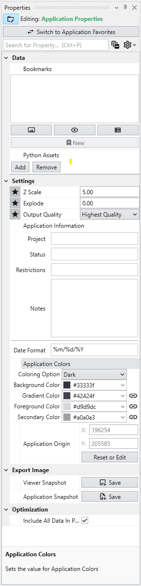
Below is the default content of Application properties.
Following is a description of each category:
Category
Property
Description
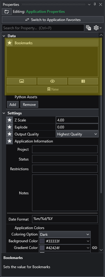
Data
Bookmarks
View and manage saved bookmarks. See Bookmarks for details.
Python Assets
Python scripts reusable from other Python files in your application. Right-clicking will generate the proper import syntax using the EVS python API, which allows these to be imported in scripts even when packaged.
Settings
Z Scale
Adjusts the vertical exaggeration of 3D data.
Explode
Controls the separation of layered data components.
Output Quality
Set the quality setting used in certain modules (e.g., Highest Quality). Allows optimization of workflow by using a low quality file while manipulating and a high quality file when producing output.
Application Information
Provides a mechanism to supply reusable metadata in various outputs and scripts. Often available as environment variables in modules which produce text, as well as used in CTWS output.
Application Colors
Customize the appearance of many module outputs by default. See Application Colors for details.
Application Origin
Defines the spatial anchor for the project coordinates. The first time a file is read, the origin will be set based off the coordinates of that data. Everything is then computed relative to the application origin from then on in order to maintain the best precision for 3d calculations. If you reuse an application and change the data, you must reset the application origin.
Reset or Edit Origin
Allows manual recalibration of the project center.
Export Image
Viewer Snapshot
Writes the contents of the viewer to an image file.
Application Snapshot
Writes the contents of the application window (the network) to an image file.
Optimization
Include All Data In Probe
When enabled, all data is included in probe results in the viewer. This uses more memory, but increases the functionality for inspecting the data.
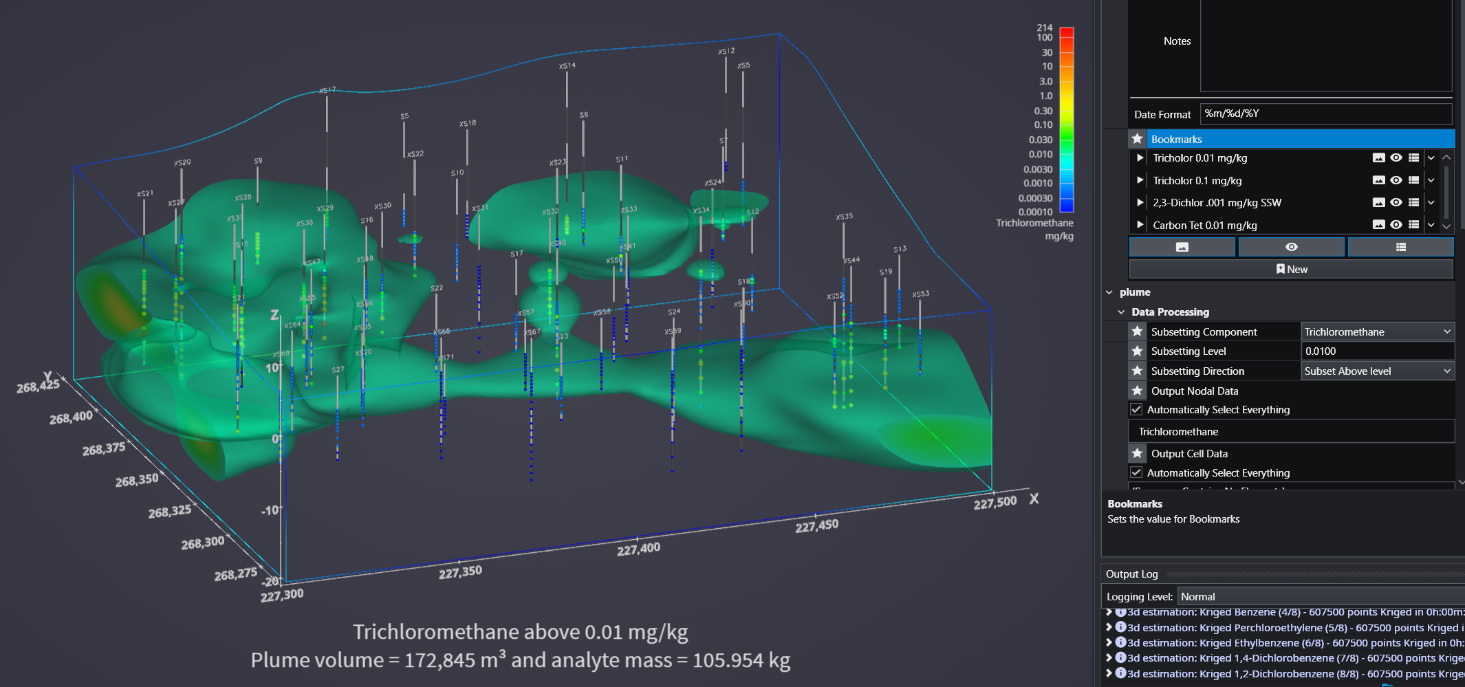
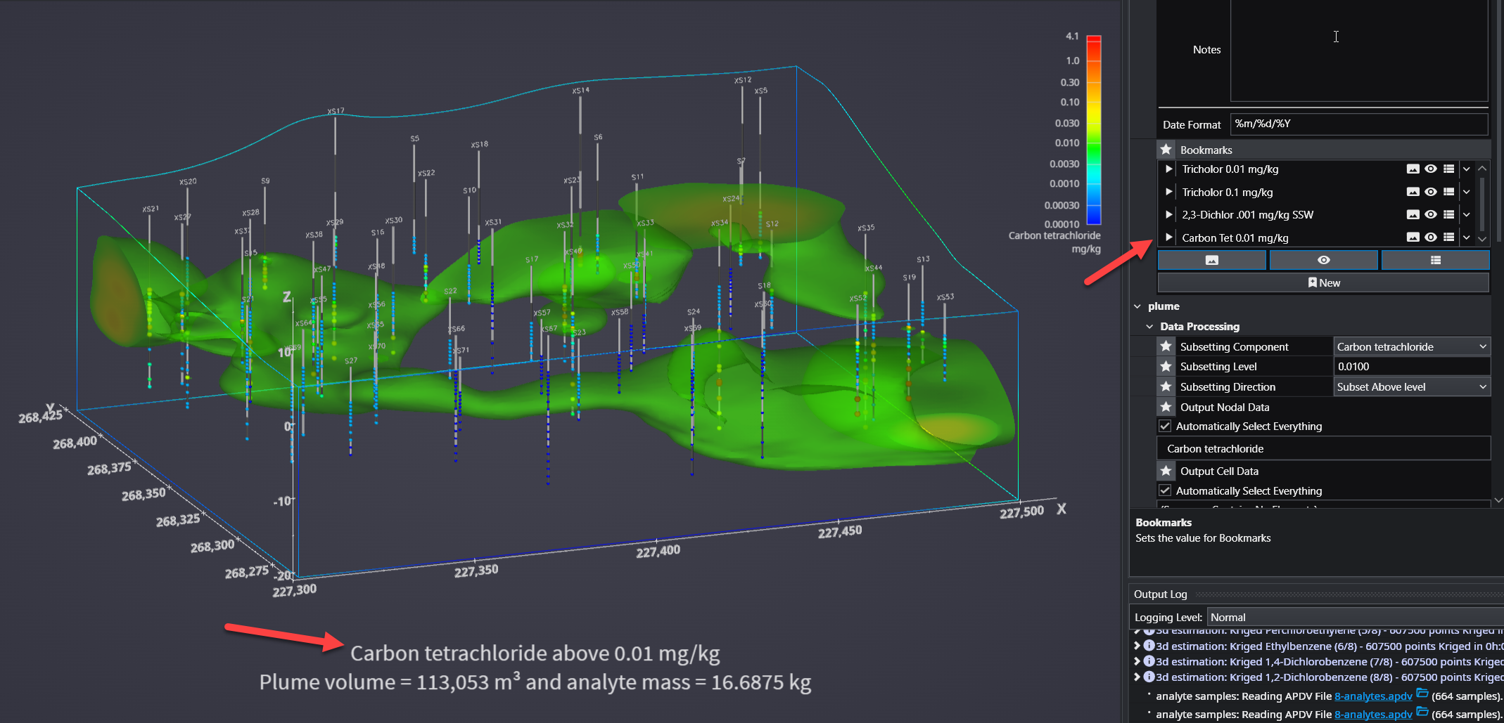
Bookmarks provide an easy way to save and recall specific configurations of your application. They act as saved “snapshots” that can instantly change the camera view, which objects are visible, and the current state of any sequences. They also export to C Tech Web Scenes.
This is essential for creating presentations, standardizing views for analysis, and optimizing the user experience in any exported C Tech Web Scenes.
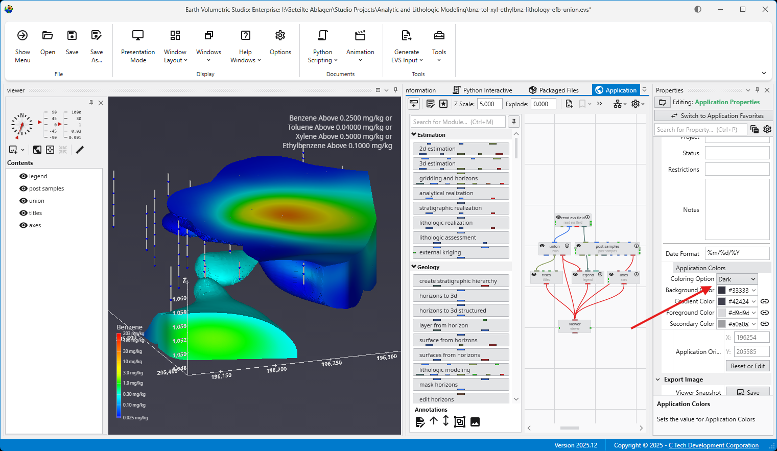
The Application Colors feature provides a centralized way to manage a consistent color palette across your entire application. By setting a few base colors, you can ensure that various annotation modules - such as titles, legends, and axes - as well as the viewer background all share a coordinated and professional look.
This feature is particularly powerful when used with linked properties, as it allows you to switch between entire color themes (e.g., from a light to a dark theme) with a single click.
Subsections of Application Properties
Bookmarks provide an easy way to save and recall specific configurations of your application. They act as saved “snapshots” that can instantly change the camera view, which objects are visible, and the current state of any sequences. They also export to C Tech Web Scenes.
This is essential for creating presentations, standardizing views for analysis, and optimizing the user experience in any exported C Tech Web Scenes.
What Bookmarks Control
A single bookmark can be configured to control one, two, or all three of the following aspects of your application:
Aspect
Description
View
The camera’s position, orientation, and zoom level in the Viewer.
Visibility
The visibility and opacity settings of all modules in the application.
Sequence State
The currently selected state of all Sequence modules.
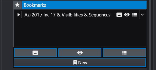
Bookmarks are created and managed from the Bookmarks panel in the Application Properties.
Follow these steps to create a new bookmark:
Set up your scene: Arrange the application to the exact state you want to save.
Adjust the camera to the desired view.
Set the visibility and opacity of each object in the Viewer.
Select the desired frame for any sequence animations.
Select Action Types: In the Bookmarks panel, click the buttons to activate the aspects you want this bookmark to control. The active buttons are highlighted in blue. From left to right, they are Views, Visibilities, and Sequence States. One or more of these must be selected to create a new bookmark.
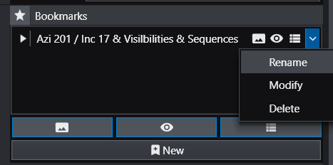
Create the Bookmark: Click the New button (the plus icon). A new bookmark will appear in the list with a default name.
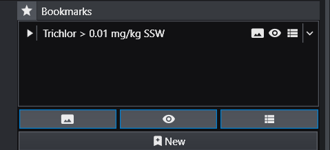
Rename the Bookmark: The default name can be generic. It is highly recommended to give it a descriptive name. Click the dropdown arrow on the far right of the bookmark and select Rename.
For example, a name like “Trichlor Plume > 0.01 mg/kg” is much more informative.
Using Bookmarks
To apply a bookmark, simply click the “Play” icon (the white triangle) next to the bookmark’s name in the list. This will instantly update the application to the saved view, visibility, and/or sequence state defined by that bookmark.
When you save your project as a C Tech Web Scene (.ctws file), these bookmarks are included, allowing others to interact with your scene in the predefined ways you have designed.
Advanced Visibility Options
When saving visibility in a bookmark, you have advanced control over how objects behave, which is especially useful for Web Scenes.
Option
Description
Locked
A “Locked” object is always visible and cannot be turned off by the user in the C Tech Web Scene Viewer. This is ideal for essential items like a site map, buildings, or a company logo that should always remain in view.
Excluded
An “Excluded” object is not written to the Web Scene at all. This is equivalent to disconnecting the module from the viewer and can be used to hide intermediate or unnecessary components from the final output.
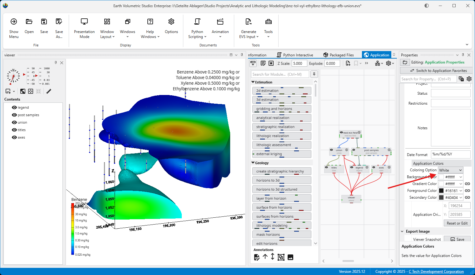
The Application Colors feature provides a centralized way to manage a consistent color palette across your entire application. By setting a few base colors, you can ensure that various annotation modules - such as titles, legends, and axes - as well as the viewer background all share a coordinated and professional look.
This feature is particularly powerful when used with linked properties, as it allows you to switch between entire color themes (e.g., from a light to a dark theme) with a single click.
Accessing Application Colors
The Application Colors settings are located in the **Application Properties**application-properties.md panel.
Color Properties and Options
The panel contains several options for defining your color scheme.
Option
Description
Coloring Option
This dropdown menu allows you to quickly switch between predefined color themes. By default, it includes “White” and “Dark” themes, which are designed for light and dark viewer backgrounds, respectively.
Interface Colors
These four properties define the core colors of your theme.
Background Color: Sets the background color of the viewer.
Gradient Color: Used with the Background Color to create a two-color gradient in the viewer background.
Foreground Color: The primary color used for text and lines in most annotation modules.
Secondary Color: A supplementary color used for secondary elements, such as shading on the compass rose in the direction_indicator module.
Linked Properties: The Key to Automatic Updates
For the Application Colors to automatically update your modules, the color properties within those modules must be linked. When a property is linked, it inherits its value from the global Application Colors settings. If you unlink a color property in a module, it will use its own manually set color and will no longer be affected by theme changes.
You can identify a linked property by the link icon next to it. For more information, see the Linked Properties topic.
Affected Modules
The following modules are designed to use the Application Colors when their color properties are linked:
Module
Usage
viewer
Uses the Background Color and Gradient Color for its background.
axes, titles, 3d_titles, legend, and 3d_legend
These modules primarily use the Foreground Color for their text and lines.
direction_indicator
This module uses the Foreground Color for its text and the Secondary Color for shading effects on elements like the compass rose.
Example of Switching Coloring Option
When the modules’ color properties are linked, changing the Coloring Option has an immediate effect on the entire scene.
The application below is using the White Coloring Option. Note the dark text and lines on the title, axes, and legend, which provide high contrast against the light background.
By simply switching the Coloring Option to Dark, all linked modules automatically update. The text and lines change to a light color to maintain contrast against the new dark viewer background.
Light and dark themes can also be toggled in the Options panel in the Menu.
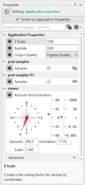
The Application Favorites feature provides a powerful way to create a custom control panel for your EVS application. It allows you to gather the most important properties from various modules and global settings into a single, centralized location within the Properties window.
Info
When creating EVS Presentations, the only properties which will be editable in the resulting Presentation Application (*.evsp) are the Application Favorites. All other properties are unavailable in an EVS Presentation.
This is especially useful in large or complex applications, as it eliminates the need to navigate to each individual module to adjust key parameters. Instead, you can manage all critical settings from one convenient view.
Accessing Application Favorites
The Application Favorites are available via a button in the Application Window toolbar:
Alternatively, you can also access these when editing the Application Properties. When the Application Properties are displayed in the Properties window, click the Switch to Application Favorites button at the top.
Finally, double clicking on the background of the network area will open the Application Favorites or Application Properties (whichever was most recently viewed).
The Application Favorites View
Once you switch to the Application Favorites view, you will see a list of all the properties you have marked with a star. The properties are organized into groups based on their source module. For example, global settings like Z Scale and Explode are listed under “Application Properties,” while module-specific properties are grouped under the name of their respective module (e.g., “viewer”).
You can edit any of these properties directly from this view, just as you would in the standard properties editor.
How to Favorite a Property
You can favorite almost any property from any module.
Select a module in the Application Network to display its parameters in the Properties window.
To favorite a property, click in the empty space to the left of its name. A star icon will appear, indicating that the property has been added to your Application Favorites.
It is important to note that this action favorites the property for that specific instance of the module, not for all modules of that type. This allows you to select different key parameters from different modules. The same property from different modules can appear in the Application Favorites at the same time.
How to Remove a Property from Favorites
To remove a favorited property, simply click the star icon in either the module or the Application Favorites again.
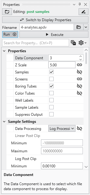
Module Properties
When you select a module in the Application Network, its settings are displayed in the Properties window. This window allows you to configure the module’s parameters and control its execution behavior. At the top of the window, the name of the module you are editing is displayed.
Switch to Display Properties
This button provides a quick way to access the properties of the module’s primary Renderable Port (red) if they are being displayed in a viewer. The Red Port Properties will also feature a button to quickly switch back again.
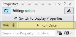
Execution Control
The toolbar at the top of the Module Properties window provides powerful tools for managing when and how a module executes.
Run Toggle: This switch controls the module’s automatic execution. By default, it is on, meaning the module will automatically run whenever one of its properties is changed or when an upstream module it depends on finishes running. Toggling this off prevents the module from running automatically. This is particularly useful when you want to make multiple changes to a module’s settings without triggering potentially time-consuming computations after each adjustment.
This is also displayed and configurable on the modules in the Application Network. See Module Status Indicators.
Run Once Button: When available, this button allows you to manually trigger the execution of the currently selected module. It forces the module to run a single time. This is most effective when the Run toggle is turned off, as it lets you apply your changes and see the result without having to re-enable automatic execution.
Module-Specific Properties
Below the execution controls, the Properties section contains all the configurable parameters for the selected module. The settings here are unique to each module’s function. These properties allow you to customize the module’s behavior to fit the specific needs of your analysis.
Property Description
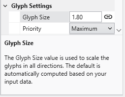
At the bottom of the Properties window is a description panel. This panel is your first and most important resource for understanding what a specific property does. When you select a property from the list, this panel automatically updates to show a detailed explanation of that property and its function. For instance, selecting “Data Processing” will display text explaining that this property allows to declare whether the input data is to be treated as linear or log processed. This immediate, context-sensitive help makes it easy to learn and configure even complex modules without having to consult external documentation.
Here is an example for the Property Description of the “Glyph Size” property:
Understanding Linked Properties
In Earth Volumetric Studio, a Linked Property is a parameter whose value is automatically determined within the application, rather than being manually set by the user. This dynamic connection allows for a more intelligent and consistent workflow. You can identify a linked property by the link icon located next to it in the Properties window
When the link icon is closed/connected, the property is linked, and its value will update automatically based on its source.
When the link icon is broken, the property is unlinked, and its value is fixed to whatever you have manually set.
You can toggle a property’s linked state by simply clicking on the link icon.
Linked Property:
Unlinked Property:
Info
Not all properties can be linked. If a property does not have a link icon next to it, it is a manual property. Its value may be set directly by the user and will not change automatically.
The Purpose of Linked Properties
Linked properties are a core feature of the EVS expert system, designed to streamline the modeling process. By linking properties, EVS can ensure consistency across your entire application, provide smart defaults based on your data, and maintain visual coherence. For example, linking the Z Scale of multiple modules to the global Application Z Scale means you only have to change it in one place, but can still unlink and override it as needed. Linked properties may also provide good automatic starting values for further unlinked manual refinement.
While you can unlink any linked property to gain manual control, it is generally recommended to keep properties linked unless you have a specific reason and understand the effect of the change. This approach leads to a faster and better-looking result.
Info
Re-linking a previously unlinked property will cause its value to revert to the automatic, context-driven setting. This change may also trigger the module to re-execute immediately to reflect the new state, unless the module’s Run toggle is turned off.
Common Categories of Linked Properties
Z Scale
This is the most common linked property and the one you should change least often. Nearly every module that deals with 3D data has a Z Scale property that is, by default, linked to the global Z Scale found in the Application Properties. This ensures that all visual components in your scene use the same vertical exaggeration, which is critical for correct spatial representation.
Colors
Many modules that create visual elements, such as titles or legends, have color properties that are linked to the global Application Colors setting. When you switch the application theme between Dark, White, or Custom, these linked colors will automatically adjust to ensure they remain visible and aesthetically pleasing against the new background color. Unlinking a color property, such as Title Color, will fix it to a specific color, and it will no longer adapt to theme changes.
Coordinates
Many modules that process spatial data have coordinate properties (e.g., Min/Max extents) that are linked to the incoming data. When the module is run, it analyzes the input field and automatically populates these properties with the correct coordinate values. If the input data changes, re-running the module will cause these linked properties to update accordingly.
Expert System Parameters
EVS includes an expert system that analyzes your data to provide intelligent, scientifically appropriate default values for complex parameters. This is most common in geostatistical modules like kriging or lithologic modeling. Parameters for kriging and variogram settings are often linked to the expert system, which suggests optimal values based on the input data. Unlinking these properties allows for manual fine-tuning but overrides the data-driven recommendations.
Port Properties
When you double-click an output port on a any module in the Application Network, the Properties window displays detailed information and settings for that specific port. While the properties shown vary depending on the type of data the port provides, certain elements are common to all ports.
At the top of the window, a Switch to Module Properties button provides a convenient way to navigate back to the properties of the module that owns the port.
Common Port Properties
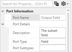
All output ports display a Port Information section with the following properties:
Renderable Object Port Properties In Earth Volumetric Studio, a red port is a Renderable Object port. It outputs a visual object—such as a surface, a set of points, or a volume—that can be displayed in a viewer. By editing the properties of this port, you can control every aspect of how the object is visualized in the 3D scene. See the Visualization Fundamentals section for additional details on rendering options.
Field Port Properties In Earth Volumetric Studio, a blue port is a Field Port. It is the most common port type and is responsible for passing grid structures and their associated data between modules. A “field” contains the geometry (nodes and cells) as well as any data values defined on that grid, such as analytical results or material properties.
Subsections of Port Properties
Renderable Object Port Properties
In Earth Volumetric Studio, a red port is a Renderable Object port. It outputs a visual object—such as a surface, a set of points, or a volume—that can be displayed in a viewer. By editing the properties of this port, you can control every aspect of how the object is visualized in the 3D scene. See the Visualization Fundamentals section for additional details on rendering options.
To access these properties, you can double-click on a red port in the Application Network, which will load its settings into the Properties window.
Port Information
General information about the port as described in the Port Properties topic.
General Properties
This is the primary section for controlling the object’s appearance, coloring, and visibility in the 3D scene.
Property
Description
Visible
A master toggle to show or hide the object in the viewer.
Pickable
Determines if the object can be selected in the viewer using the probe tool (Ctrl + Left-click). Disabling this can be useful for large, transparent objects that might interfere with selecting objects behind them.
Opacity
Controls the transparency of the object. A value of 100% makes the object fully opaque, while 0% makes it completely invisible.
Faces To Display
Controls which faces of a 3D object are rendered.
Display All: Renders both the front and back sides of faces.
Camera Facing: Renders only the faces pointing toward the camera. This is useful for making closed transparent objects look correct and can improve performance.
Facing Away: Renders only the faces pointing away from the camera.
Color By
Determines the source of the object’s color.
Nodal Data: Colors the object based on data values at the nodes, often resulting in smooth color gradients.
Cell Data: Applies a uniform color to each entire cell based on its data value.
Solid Color: Applies a single, uniform color to the entire object.
Node Data / Cell Data
If coloring by data, these dropdowns let you select which specific data component to use for coloring.
Vector Component / Use Vector Magnitude
If the selected data is a vector, this allows you to color the object by a single component or by the vector’s overall magnitude.
Node/Cell Data Datamap
Opens the datamap editor to define the mapping between data values and colors. See the Datamaps topic for more information.
Object Color
If Color By is set to Solid Color, this control allows you to select the specific color for the object.
Object Secondary Color
This color is primarily used for drawing the outlines of cells when “Hide Cell Outlines” is disabled.
Normals Generation
Affects how lighting is calculated on surfaces.
Default: Selects the best method based on the input data type.
Cell Normals: Results in flat shading with hard transitions between cells.
Point Normals: Averages normals at each point, creating a smooth, continuous appearance.
Rendering Priority
A numeric value that influences the drawing order of objects. Objects with higher numbers are drawn later (on top of others).
Export Properties
This section contains settings related to exporting the application.
Property
Description
Exclude From Compression
If checked, this object’s geometry will not be compressed when exporting to a C Tech Web Scene. This preserves full precision but can result in a significantly larger file size.
Advanced Properties
These settings provide fine-grained control over geometry processing and rendering. They are intended for advanced users and should generally be left at their default values unless you are addressing a specific rendering issue.
Rendering Modes
This section controls how different geometric components of the object are displayed.
Property
Description
Point/Line/Surface/Volume/Bounds Display Mode
Each dropdown allows you to change the rendering style for a specific component (e.g., render a surface as a wireframe (Lines) or display points as spheres (Glyphs)).
Hide Cell Outlines
Toggles the visibility of the wireframe edges of the cells that make up the object.
Surface Properties
These properties control how the object’s surface interacts with light in the scene. They are intended for advanced users and should generally be left at their default values unless you are addressing a specific rendering issue.
Property
Description
Ambient
Controls how much ambient light the surface reflects (the object’s color in the absence of direct light).
Diffuse
Controls how much light the surface reflects from direct light sources, determining the primary illuminated color.
Specular
Controls the color of specular highlights (bright spots where light reflects directly toward the camera).
Gloss
Controls the size and intensity of specular highlights. Higher values create smaller, sharper highlights, making the surface appear shinier.
Point And Line Properties
This section contains settings that apply specifically to objects composed of points or lines.
Property
Description
Line Style
Sets the pattern for lines.
Solid: A continuous, unbroken line.
Dashed: A line made of a series of short segments.
Dotted: A line made of a series of dots.
**Dashed-Dotted: **A combination of the Dashed and Dotted line styles.
Line Thickness
Controls the width of lines in pixels. A value of 0 uses a default, fast-rendering single-pixel line.
Glyph Size
If points or lines are rendered as glyphs (e.g., quads), this controls their size.
Smooth Lines
Toggles anti-aliasing for lines. When enabled, lines will appear smoother with less jaggedness.
Texture Settings
If the object has a texture applied, these properties control how it is mapped and rendered. They are intended for advanced users and should generally be left at their default values unless you are addressing a specific rendering issue.
Property
Description
Interpolation
Determines how the texture is sampled when magnified or minified. Bilinear (default) averages the four nearest texels for a smooth but potentially blurry appearance.
Tile
Controls the texture’s behavior at its boundaries. Clamp causes the edge pixels to be stretched to fill the rest of the surface.
Blending
Defines how the texture’s color is combined with the object’s underlying color. Replace causes the texture’s color to completely overwrite the object’s original color.
Type
Relates to the use of mipmaps. Single Level indicates that only the original, full-resolution texture is used, without any lower-resolution versions for distant objects.
Field Port Properties
In Earth Volumetric Studio, a blue port is a Field Port. It is the most common port type and is responsible for passing grid structures and their associated data between modules. A “field” contains the geometry (nodes and cells) as well as any data values defined on that grid, such as analytical results or material properties.
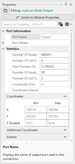
To access the properties of a Field Port, you can double-click on any blue port in the Application Network. This will load its settings and summary information into the Properties window.
Port Information
General information about the port as described in the Port Properties topic.
Statistics
This section gives a high-level summary of the contents of the field.
Property
Description
Number Of Nodes
The total count of nodes (points) that define the field geometry.
Number Of Cell Sets
The number of distinct groups of cells. Cell sets are often used to represent different geologic layers or materials.
Total Number Of Cells
The total count of all cells across all cell sets in the field.
Number Of Node Data / Number Of Cell Data
The count of different data components attached to the nodes or cells.
Coordinate Units
The measurement unit for the grid’s coordinates (e.g., meters, feet).
Coordinate Extents
The overall dimensions (X, Y, Z) of the grid’s bounding box.
Coordinates
This table displays the minimum and maximum coordinate values for the X, Y, and Z axes, defining the spatial bounding box of the grid. The Z (Scaled) value reflects the coordinates after any global Z Scale has been applied.
Summary Statistics
This section provides a quick statistical overview of a selected data component within the field.
Property
Description
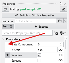
Data Component
A dropdown menu to select which data component you wish to analyze.
Data Units
The measurement unit for the selected data component.
Is Log
A checkbox indicating if the data is on a logarithmic scale.
Data Min / Data Max
The minimum and maximum values for the selected data component.
Histogram
A small histogram plot provides a quick visual summary of the data’s distribution.
Open Statistics Window
This button launches a separate, more detailed window for in-depth statistical analysis.
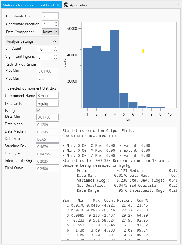
The Statistics Window
The Statistics Window provides a comprehensive and interactive environment for analyzing the data within a field. It is composed of several panels that allow you to customize the analysis and view detailed statistical results, both graphically and textually.
Panel / Component
Description
Analysis Settings
Located in the top-left corner, this panel allows you to control how the statistical analysis is performed and displayed.
Bin Count: Adjusts the number of columns in the histogram to change the granularity of the distribution plot.
Significant Figures: Controls the precision of the displayed numerical results.
Restrict Plot Range: When enabled, allows you to manually define the minimum and maximum values for the analysis.
Selected Component Statistics
Located below the analysis settings, this panel presents key statistical metrics for the chosen data component.
Data Mean: The average value.
Data Median: The middle value of the dataset.
Standard Dev.: The standard deviation, a measure of data dispersion.
Interquartile Rng.: The range between the first and third quartiles.
Histogram Plot
The main area on the right, providing a clear visual representation of the data’s distribution by showing the number of data values (Counts) that fall into each bin.
Statistics Summary
A text-based report below the plot, offering a summary of coordinate extents and a detailed breakdown of the statistics.
Bin Data Table
Located at the bottom, this table lists the specific data for each bin, including its minimum and maximum range, the count of values it contains, and the cumulative percentage of the total data set.
Introduction to Datamaps
In the fields of scientific and geometric visualization, a datamap is a fundamental concept that serves as the bridge between raw numerical data and its visual representation. At its core, a datamap is a function or a lookup table that translates data values into visual properties, most commonly color. Think of it as a sophisticated legend that instructs the rendering engine how to “paint” the data onto a geometric object, such as a surface, a volume, or a set of points.
Every value in your dataset, whether it represents temperature, contaminant concentration, pressure, or a geologic material type, is assigned a color based on the rules defined in the datamap. This transformation is what turns an abstract collection of numbers into an intuitive and immediately understandable visual model. Without datamaps, a 3D model of contaminant distribution would be a colorless, featureless shape, providing no insight into where the highest concentrations are or how they vary in space. The datamap is what brings the data to life, allowing us to see the patterns, trends, and anomalies that would otherwise be hidden in spreadsheets and data files.
The Purpose of Datamaps in EVS
In Earth Volumetric Studio, datamaps are the primary tool for communicating the meaning of your data within a visual context. Their purpose extends beyond simply making things colorful; they are a critical component of data analysis and presentation for several key reasons.
First, they make complex data interpretable. A bright red area in a plume model is instantly recognizable as a “hotspot” of high concentration, while a transition from green to blue can clearly show the gradient where values are decreasing.
Second, they provide a quantitative reference. A well-designed datamap, coupled with a legend, ensures that the visualization is not just a pretty picture but a scientifically accurate representation. Each color corresponds to a specific data value or range, allowing a viewer to probe any point on a model and understand its precise quantitative meaning.
Finally, they are essential for highlighting features of interest. Data in environmental and geological sciences often spans many orders of magnitude. A datamap can be carefully designed to focus the visual contrast on the most critical parts of the data range, making subtle but important variations stand out while de-emphasizing less relevant data.
Types of Data and Datamap Processing
Datamaps in EVS are highly flexible and can be configured to handle different types of data and distributions. The way a datamap translates values to color can be linear, non-linear, or categorical.
Linear Datamaps
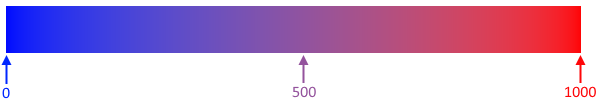
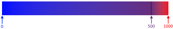
A linear datamap applies a smooth, uniform color gradient across the entire range of the data. The relationship between a data value and its position in the color gradient is a straight line. For example, in a dataset ranging from 0 to 1000, a value of 500 would be mapped to the exact middle of the color ramp. This type of mapping is best suited for data that is evenly distributed and where the importance of changes is consistent across the entire range, such as a simple temperature scale.
Non-Linear Datamaps
A non-linear datamap is used when the data is not uniformly distributed or when certain ranges are more important than others. In this case, the relationship between data values and colors is not a straight line. This allows you to allocate more “color space” to the most critical parts of your data range.
A classic example is contaminant concentration data, which might range from 0.01 to 10,000. If a linear datamap were used, most of the color gradient would be dedicated to the high-end values, making it impossible to distinguish between low-level concentrations (e.g., 0.1 vs. 1.0), which might be the most critical range for regulatory purposes. A non-linear datamap can be configured to stretch the color gradient across the lower values, providing high visual contrast where it is needed most.
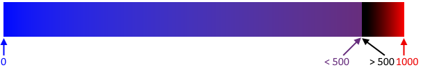
The colors of breaks on both sides don’t have to be continuous. If the Lock Adjacent Breaks toggle in the Datamap Editor is disabled, you can choose both colors separately.
A note on precision: Due to the nature of precision in floating-point calculations, a value that is identical to a break point can be categorized into either the adjacent upper or lower interval. If you need to ensure a specific value is colored correctly, we recommend slightly shifting the break point. For example, changing a break from 500.0 to 500.0001 ensures the value 500.0 falls into the lower interval.
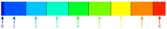
Categorical Data
Datamaps are also used for categorical data, which is qualitative rather than quantitative. Examples include geologic material types (“Sand”, “Clay”, “Gravel”), land-use classifications, or sample location IDs. For this type of data, the datamap assigns a single, discrete color to each unique category. There is no gradient or blending between colors. In EVS, this is typically handled by assigning an integer ID to each category (e.g., Sand=1, Clay=2). The datamap is then configured with distinct colors for each integer value, effectively creating a color key for your categorical data.
Logarithmic Processing
Logarithmic processing is a specific type of non-linear mapping designed for data that spans several orders of magnitude. By taking the logarithm of the data values before mapping them to color, vast ranges are compressed into a more manageable scale. This makes logarithmic datamaps the standard and most effective way to visualize data like hydraulic conductivity or contaminant concentrations. EVS handles this transformation automatically when the log processing option is selected in many modules, so you do not need to manually convert your data. The datamap works with the log-transformed values, but associated legends will still display the original, human-readable values.
The Datamap Editor is the primary tool in Earth Volumetric Studio for creating and customizing the mapping between your data values and the colors used to represent them in a visualization. It provides a powerful, interactive interface to control color gradients, data ranges, and scaling, allowing you to effectively highlight the features of interest in your data.
Subsections of Datamaps
The Datamap Editor is the primary tool in Earth Volumetric Studio for creating and customizing the mapping between your data values and the colors used to represent them in a visualization. It provides a powerful, interactive interface to control color gradients, data ranges, and scaling, allowing you to effectively highlight the features of interest in your data.
You can access the Datamap Editor by clicking the Edit button next to the Node Data Datamap or Cell Data Datamap properties in a module’s rendering settings.
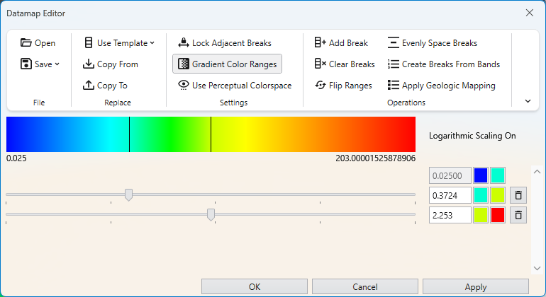
The editor is composed of three main areas: the toolbar at the top, the color ramp preview in the middle, and the color break editor at the bottom.
Toolbar
The toolbar provides access to file operations, settings, and tools for manipulating the datamap.
File and Replace Operations
Operation
Description
Open
Allows you to load a previously saved datamap configuration from a .CTDmap file, enabling you to reuse complex color schemes across different projects and models.
Save
This dropdown menu provides two distinct ways to save the current datamap configuration to a .CTDmap file.
Save As Generic: Saves the datamap with its breaks defined by their relative positions (e.g., percentages). This makes the saved datamap a flexible template that will adapt to a new dataset’s minimum and maximum values.
Save With Values: Saves the datamap with its breaks locked to their current, fixed data values. This is useful for applying a consistent color mapping to multiple datasets that share the same data extents or have specific, meaningful thresholds.
Use Template
Applies one of the default datamap templates, such as Default Node Map, Linear Grayscale, or perceptually uniform scientific colormaps.
Copy From
Opens a dialog to copy a datamap from another module in your application, allowing you to select a specific source and apply its datamap to the current module.
Copy To
Performs the reverse of Copy From. It allows you to apply the current datamap’s configuration to one or more selected modules and ports.
Settings
Setting
Description
Lock Adjacent Breaks
This toggle locks the colors between breaks. When enabled, changing the color of a break point will also update the adjacent break point in the next range, ensuring a continuous color gradient.
Gradient Color Ranges
This toggle controls whether to use smoothly changing colors. When enabled, colors blend seamlessly between break points. When disabled, each range is filled with a single, solid color.
Use Perceptual Colorspace
This option switches the color interpolation method to a “visual perceptual colorspace,” which can produce gradients that are perceived as more uniform and natural by the human eye.
Operations
Operation
Description
Add Break
Adds a new break position to the datamap, allowing you to introduce a new color and data value point to refine your color gradient.
Evenly Space Breaks
Redistributes all existing color breaks linearly across the full data range, creating a uniform gradient.
Clear Breaks
Removes all intermediate color breaks, leaving only the start and end points and creating a simple, two-color gradient.
Create Breaks From Bands
Automatically creates new color breaks at the exact data values used by another module (like isolines), ensuring color changes align perfectly with contour lines or other banded visualizations.
Flip Ranges
Reverses the color ramp, so that the color previously at the maximum value is now at the minimum value, and vice-versa.
Apply Geologic Mapping
Designed for categorical data, this function creates a series of discrete, solid color ranges corresponding to the integer IDs used to represent different geologic materials.
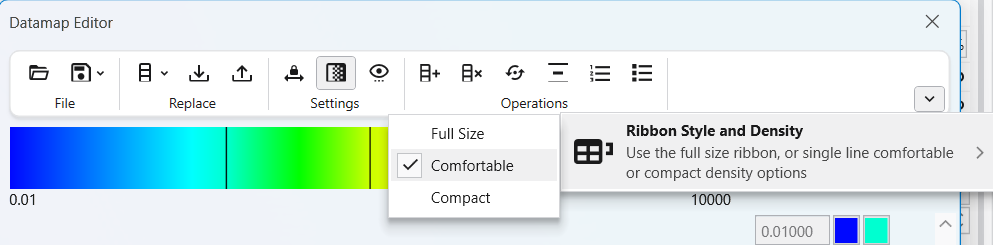
The toolbar also has similar options to the EVS Main Toolbar in terms of display style and density.
Color Ramp and Break Editor
This is the main interactive part of the editor where you define the datamap.
Color Ramp Preview: The large horizontal bar shows a preview of the final datamap. It displays the colors and the smooth transitions between them, based on the color breaks you have defined below it. The minimum and maximum data values of the current range are displayed at the ends of the ramp.
Logarithmic Scaling Indicator: Text such as “Logarithmic Scaling On” will appear to the right of the color ramp. This indicates that the datamap is currently processing the data on a logarithmic scale. This is essential for effectively visualizing data that spans several orders of magnitude, as it allocates more color variation to the lower-end values.
Color Break Editor: This section is where you define the specific points of your datamap. The datamap is composed of one or more color intervals, and the points that define the start and end of these intervals are called color breaks. Within each interval, the color transitions in a linear gradient based on the data values and colors set at its start and end breaks. A key feature of the editor is that the color at the end of one interval does not need to be continuous with the color at the start of the next. By disabling the Lock Adjacent Breaks setting, you can create a “hard break,” or an abrupt change in color at a specific data value. This is useful for visually separating distinct data ranges. Furthermore, the length of each interval can be adjusted independently, allowing you to create a non-linear datamap by stretching or compressing the color gradient across different parts of the data range.
Each color break is represented by a row in the editor, which includes:
Component
Description
Data Value Input Box
Allows for precise numeric entry of the data value for the break.
Color Swatch
Opens a color picker to set the color for the break.
Slider
Provides interactive adjustment of the data value for the break.