The Tools menu provides a collection of utilities for file conversion, data processing, and creating animations. These tools are designed to help you prepare your data for use in EVS.
Accessing Tools
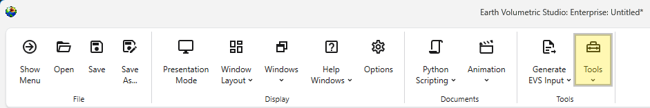
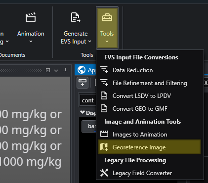
The Tools button can be found in the Main Toolbar. Clicking it will open a list of available tools.
Tool Buttons
EVS Input File Conversions
This section contains tools for processing and converting various data files into formats optimized for EVS.
Tool
Description
Data Reduction
This utility helps you manage large datasets by reducing the number of data points. It can be used to sample or filter your data, which can improve application performance and reduce processing times with configurable loss of detail. It is used to get optimal results when kriging dense data. See the Dense Data tutorial video.
File Refinement and Filtering
Use this tool to clean and refine your data files. It allows you to apply filters to remove outliers, correct errors, or extract a specific subset of your data based on defined criteria, ensuring higher quality input for your models.
This tool converts the Borehole Geology(.geo) file format into the Geology Multi-File (.gmf) format. This is useful if you want to replace a single surface in a GEO hierarchy (such as the ground surface) with more high-resolution data that is not synchronous with your .GEO borings.
Image and Animation Tools
This group of tools helps you create animations and prepare images for use in your projects.
Tool
Description
Images to Animation
This utility takes a sequence of individual image files and compiles them into a single animation video. This is useful for creating time-lapse visualizations of your models or other dynamic presentations.
Georeference Image
Creates and edits world files or .gcp (ground control point) files for images. Use this tool to assign real-world geographic coordinates to a raster image, such as an aerial photograph or a scanned map. Georeferencing allows the image to be accurately positioned and scaled within your 3D scene alongside other spatial data.
Legacy File Processing
This section provides tools for working with older, outdated file formats.
Tool
Description
Legacy Field Converter
Reads older format files that can contain EVS Fields, such as Field (.FLD), UCD (.INP) and netCDF files (.CDF) and converts them to standard EVS Field File format (.EFB). The .EFB format is used because it is the smallest and old file formats do not require the more complex features that the .EF2 format allows.
The Images To Animation tool allows you to compile a sequence of individual image files into a single video animation. This is ideal for creating time-lapse visualizations, showcasing model changes over time, or presenting a series of related images, for example written by EVS through sequences and Python Scripting, as a dynamic video.
The Georeference Image tool is a useful utility for assigning real-world geographic coordinates to raster images. This process, known as georeferencing, allows you to accurately overlay images with other spatial data in your project. The tool enables you to create and edit world files (e.g., .jgw, .tfw) or ground control point files (.gcp), which store the image’s location, scale, and orientation information.
Subsections of Tools
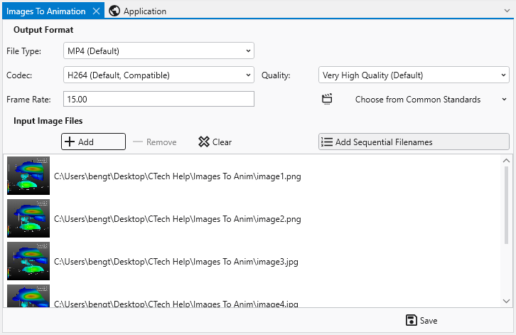
The Images To Animation tool allows you to compile a sequence of individual image files into a single video animation. This is ideal for creating time-lapse visualizations, showcasing model changes over time, or presenting a series of related images, for example written by EVS through sequences and Python Scripting, as a dynamic video.
Before creating your animation, you can configure the output settings to meet your specific needs for quality, file size, and compatibility.
Setting
Description
Frame Rate
Determines the number of frames (images) displayed per second. You can enter a custom value or select from standard presets:
60 FPS
30 FPS
NTSC (29.97 FPS)
PAL (25 FPS)
File Type
Lets you choose the container format for your output video file.
MP4 (Default): A widely supported modern option with a good balance of quality and file size.
AVI: An older, less compressed option that may result in larger files.
WebM: An open-source choice designed for web use, providing efficient compression.
Quality
Controls the trade-off between visual quality and file size.
Lossless: Preserves the exact quality of the source images but results in very large files.
Very High & High Quality: Produce excellent quality with efficient compression.
Medium & Low Quality: Offer progressively more compression for smaller file sizes, with some loss of visual detail.
Codec
Determines the compression algorithm used to encode your video.
H264: A highly compatible codec supported by most devices and platforms.
H265: A newer codec offering better compression than H264, resulting in smaller file sizes for the same quality.
H264RGB: A variant of H264 that preserves full color information, ideal for technical or scientific visualizations.
Managing Files
The File List section is where you add and manage the images that will make up your animation.
Function
Description
The File List View
This area displays the list of images you have added. Each entry shows a small preview thumbnail of the image on the left and its full file path on the right. The order of the files in this list determines the sequence in which they will appear in the final animation.
Adding and Removing Files
To add images, click the Add button to open a file dialog, where you can browse for and select one or more files. To remove a specific image, select it from the list and click the Delete button. The Clear button will remove all images from the list, allowing you to start over.
Adding Sequential Filenames
When the Add Sequential Filenames toggle is enabled, the behavior of the Add button is modified to streamline the import of numbered image sequences. If you select a single file that has a number at the end of its name (e.g., image1.png), the tool will automatically search for and add all other files in the same directory that share the same base name and have a matching extension (e.g., image2.png, image3.png, etc.).
Note that this feature requires both the file extension and the base filename (the part before the number) to match exactly. For example: Adding image1.png would add image2.png, but not image3.jpg because of its differing extension. |
About source image sizes
You may encounter a warning messages about image dimensions during conversion. This occurs because most video codecs require the dimensions of the video frame (both width and height) to be even numbers. This requirement is due to the way video compression algorithms process images. If a source image has an odd dimension, the encoder may not be able to process it. To ensure compatibility, the Images to Animation tool will automatically resize the image to the nearest even resolution before adding it to the video. While this automatic resizing is necessary for the video encoding process, it may result in a slight loss of image quality or the softening of fine features in the image.
The Georeference Image tool is a useful utility for assigning real-world geographic coordinates to raster images. This process, known as georeferencing, allows you to accurately overlay images with other spatial data in your project. The tool enables you to create and edit world files (e.g., .jgw, .tfw) or ground control point files (.gcp), which store the image’s location, scale, and orientation information.
When you launch the tool, you will first be prompted to open an image file. Once loaded, the main interface provides all the necessary functions to link pixel coordinates on the image to known map coordinates.
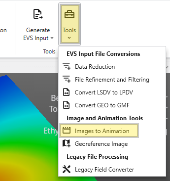
Accessing the Georeference Image tool
The Georeference Image tool can be opened from the main Tools tab in the Main Toolbar.
Interface Overview
The Georeference Image tool is organized into several key areas:
Component
Description
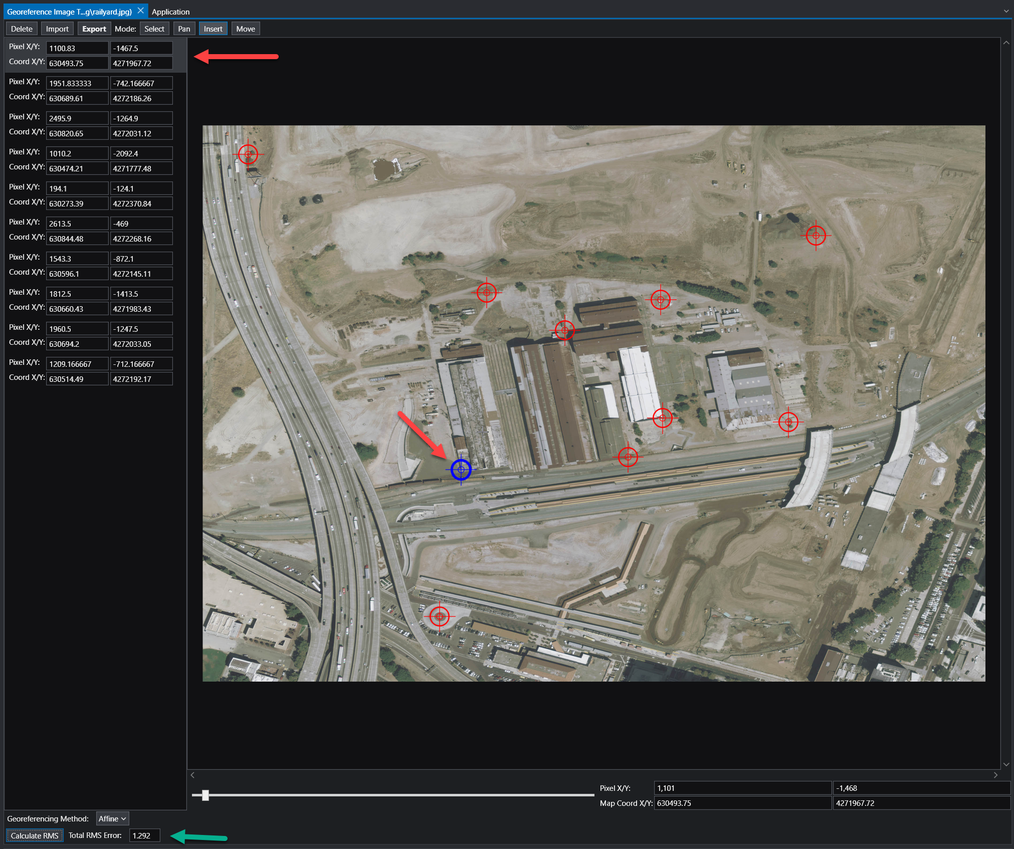
Image Panel
The central part of the window displays your image. This is your primary workspace for viewing the image and placing, selecting, and moving ground control points.
GCP List
The panel on the left lists all the Ground Control Points (GCPs) for the current image. Each point has an entry showing its pixel coordinates (Pixel X/Y) and the corresponding map coordinates (Coord X/Y).
Toolbar
Located at the top, the toolbar provides access to the main functions for managing GCPs and the georeferencing process.
Status Bar
The area at the bottom of the window displays important information, including the georeferencing method, accuracy metrics, and live coordinate readouts for your cursor’s position.
Workflow: How to Georeference an Image
Georeferencing involves creating links between points on the image and their known real-world coordinates. These links are called Ground Control Points (GCPs).
Choose a Georeferencing Method:
Use the Georeferencing Method dropdown in the status bar to select the mathematical model that will be used to transform the image from pixel coordinates to map coordinates. The best method depends on the quality of the image and the number of GCPs you have. The available methods are:
Map to Min/Max: Stretches the image to fit a bounding box defined by two GCPs representing the minimum and maximum map coordinates. Requires 2 GCPs.
Translate: Shifts the entire image based on the location of a single GCP without any rotation or scaling. Requires 1 GCP.
2 Point Translate / Rotate: Moves and rotates the image to align with two GCPs, but does not perform any scaling. Requires 2 GCPs.
Translate / Scale: Moves and uniformly resizes the image to fit two GCPs, but does not perform any rotation. Requires 2 GCPs.
Affine: A first-order polynomial transformation that can perform translation, scaling, rotation, and skewing. This is a versatile and common method for standard georeferencing. Requires a minimum of 3 GCPs. This is the recommended option, but requires at least 3 GCP points to be specified.
2nd, 3rd, and 4th Order: These are higher-order polynomial transformations used to correct for more complex, non-linear distortions in an image (e.g., lens distortion or terrain relief). They require progressively more GCPs (a 2nd Order transformation needs at least 6 GCPs) and should be used when a simpler model like Affine is not sufficient.
Add Ground Control Points:
Set the Mode on the toolbar to Insert.
Zoom and pan to a recognizable feature on the image (e.g., a road intersection, a building corner).
Click on the feature. A new entry will be created in the GCP in the list on the left of the pixel location selected.
Alter the X/Y coordinates to your desired real-world coordinates.
Repeat this process for several points distributed across the image.
Review Accuracy:
Once you have enough GCPs for your chosen method, click the Calculate RMS button. The Total RMS Error value will update. This value represents the root mean squared error, which is a measure of the average distance between the true map locations of your GCPs and their calculated locations based on the current transformation. A lower RMS error indicates a more accurate fit.
Export the Georeference File:
When you are satisfied with the accuracy, click the Export button on the toolbar. This will save the coordinate information to a file (e.g., a world file or a .gcp file) that accompanies your image.
NOTE: In general, add as many control points as possible. More control points will almost always result in a better georeferencing, as any error due to precision will be averaged out across all of the entered control points. Our recommendation is to use an Affine transformation method (which is typically the industry standard) with as many control points as possible. While three is the minimum required, ten or more is typically recommended.
Toolbar Functions
Function
Description
Delete
Deletes the currently selected GCP.
Import
Loads GCPs from an existing file (e.g., a .gcp file).
Export
Saves the current set of GCPs to a world file or .gcp file. The .gcp files are compatible with ArcGIS image link files.
Mode
Select: Allows you to select a GCP from the list or by clicking it on the image.
Pan: Allows you to pan around the image by clicking and dragging. You can also pan using the middle mouse button.
Insert: Enables you to add new GCPs by clicking on the image.
Move
Allows you to adjust the position of a selected GCP. After clicking this button, select a GCP and click its new desired location on the image to update its pixel coordinates.
Interpreting Coordinates
Once an image is georeferenced, you can use the tool to find the map coordinates of any point. As you move your cursor over the image, the Pixel X/Y and Map Coord X/Y displays in the status bar will update in real-time, showing the pixel location and the corresponding calculated geographic coordinate.