external faces

The external faces module extracts external faces from a 2D or 3D field for rendering. It produces a mesh of only the external faces of each cell set of a data set. Because each cell set’s external faces are created, there may be faces that are seemingly internal (vs. external). This is especially true when external faces is used subsequent to a plume module on 3D (volumetric) input.

Ports

Properties

External Faces

external edges

The external edges module produces a wireframe representation of an unstructured cell data mesh. This is generally used to visualize the skeletal shape of the data domain while viewing output from other modules, such as plumes and surfaces, inside the unstructured mesh. It produces a mesh of only the external edges which meet the edge angle criteria for each cell set of a data set. Because each cell set’s external faces are used, there may be edges that are seemingly internal (vs. external). This is especially true when external edges is used subsequent to a plume module on 3D (volumetric) input.

Ports

Properties

cross section

The cross section module creates a fence diagram along a user defined (x, y) path. The fence cross-section has no thickness (because it is composed of areal elements such as triangles and quadrilaterals), but can be created in either true 3D model space or projected to 2D space.

It receives a 3D field (with volumetric elements) into its left input port and it receives lines or polylines (from draw lines, polyline processing, import cad, isolines, import vector gis, or other sources) into its right input port. Its function is similar to buffer distance, however it actually creates a new grid and does not rely on any other modules (e.g. plume or plume shell) to do the “cutting”. Only the x and y coordinates of the input (poly)lines are used because cross section cuts a projected slice that is z invariant. The module recalculates when either input field is changed (and Run Automatically is on) or when the “Run Once” button is pressed.

If you select the option to “Straighten to 2D”, cross section creates a straightened fence that is projected to a new 2D coordinate system of your choice. The choices are XZ or XY. For output to ESRI’s ArcMAP, XY is required.

NOTE: The beginning of straightened (2D) fences is defined by the order of the points in the incoming line/polyline. This is done to provide the user with complete control over how the cross-section is created. However, if you are provided a CAD file and you do not know the order of the line points, you can export the CAD file using the write lines module which provides a simple text file that will make it easy to see the order of the points.

Ports

Properties

slice

The slice module allows you to create a subset of your input which is of reduced dimensionality. This means that volumetric, surface and line inputs will result in surface, line and point outputs respectively. This is unlike cut which preserves dimensionality.

The slice module is used to slice through an input field using a slicing plane defined by one of four methods:

1. A vertical plane defined by an X or Easting coordinate
2. A vertical plane defined by a Y or Northing coordinate
3. A Horizontal plane defined by a Z coordinate
4. An arbitrarily positioned Rotatable plane which requires a 3D point through which the slicing plane passes, a Dip direction, and a Strike direction

Ports

Properties

Slice Settings

Data Mapping

isolines

The isolines module is used to produce lines of constant (iso)value on a 2D surface (such as a slice plane), or the external faces of a 3D surface, such as the external faces of a plume. The input data for isolines must be a surface (faces), it cannot be a volumetric data field. If the input is the faces of a 3D surface, then the isolines will actually be 3D in nature. Isolines can automatically place labels in the 2D or 3D isolines. By default isolines are on the surface (within it) and they have an elevated jitter level (1.0) to make them preferentially visible. However they can be offset to either side of the surface.

Ports

Properties

Isoline Settings

Label Settings

cut

The cut module allows you to create a subset of your input which is of the same dimensionality. This means that volumetric, surface, line and point inputs will have subsetted outputs of the same object type. This is unlike slice which decreases dimensionality.

The cut module cuts through an input field using a cutting plane defined by one of four methods:

1. A vertical plane defined by an X or Easting coordinate
2. A vertical plane defined by a Y or Northing coordinate
3. A Horizontal plane defined by a Z coordinate
4. An arbitrarily positioned Rotatable plane which requires a 3D point through which the cutting plane passes, a Dip direction, and a Strike direction

The cutting plane essentially cuts the data field into two parts and sends only the part above or below the plane to the output ports (above and below are terms which are defined by the normal vector of the cutting plane). The output of cut is the subset of the model from the side of the cut plane specified.

Ports

Properties

Cut Settings

Data Mapping

plume

The plume module creates a (same dimensionality) subset of the input, regardless of dimensionality. What this means, in other words, is that plume can receive a field (blue port) model with cells which are points, lines, surfaces and/or volumes and its output will be a subset of the same type of cells.

This module should not normally be used when you desire a visualization of a 3D volumetric plume but rather when you wish to do subsequent operations such as analysis, slices, etc.

Ports

Properties

Data Processing

Sequence Settings

intersection

The intersection module is a powerful module that incorporates some of the characteristics of plume, yet allows for any number of volumetric sequential (serial) subsetting operations.

The functionality of the intersection module can be obtained by creating a network of serial plume modules. The number of analytes in the intersection is equal to the number of plume modules required.

The intersection of multiple analytes and threshold levels can be equated to the answer to the following question (example assumes three analytes A, B & C with respective subsetting levels of a, b and c):

“What is the volume within my model where A is above a, AND B is above b, AND C is above c?”

The figure above is a Boolean representation of 3 analyte plumes (A, B & C). The intersection of all three is the black center portion of the figure. Think of the image boundaries as the complete extents of your models (grid). The “A” plume is the circle colored cyan and includes the green, black and blue areas. The intersection of just A & C would be both the green and black portions.

Ports

Properties

Subsetting Values

union

The union module is a powerful module that automatically performs a large number of complex serial and parallel subsetting operations required to compute and visualize the union of multiple analytes and threshold levels. The functionality of the union module can be obtained by creating a network fragment composed of only plume modules. However as the number of analytes in the union increases, the number of plume modules increases very dramatically. The table below lists the number of plume modules required for several cases:

From the above table, it should be evident that as the number of analytes in the union increases, the computation time will increase dramatically. Even though union appears to be a single module, internally it grows more complex as the number of analytes increases.

The union of multiple analytes and threshold levels can be equated to the answer to the following question (example assumes three analytes A, B & C with respective subsetting levels of a, b and c):

“What is the volume within my model where A is above a, OR B is above b, OR C is above c?”

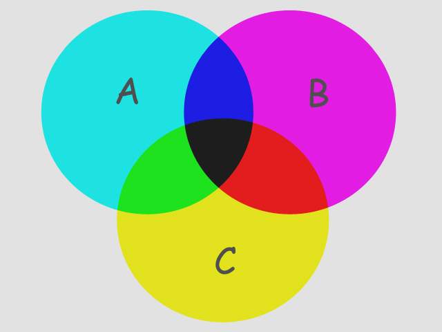
The figure above is a Boolean representation of 3 analyte plumes (A, B & C). The union of all three is the entire colored portion of the figure. Think of the image boundaries as the complete extents of your models (grid). The “A” plume is the circle colored cyan and includes the green, black and blue areas. The union of just A & C would be all colored regions EXCEPT the magenta portion of B.

Ports

Properties

Subsetting Values

subset by expression

The subset by expression module creates a subset of the input grid with the same dimensionality. It can receive a field (blue port) model with cells which are points, lines, surfaces and/or volumes and its output will be a subset of the same type of cells.

Subset by expression is different from plume in that it outputs entire cells making its output “lego-like”.

It uses a mathematical expression allowing you to do complex subsetting calculations on coordinates and multiple data components with a single module, which can dramatically simplify your network and reduce memory usage. It has 2 floating point variables (N1, N2) which are setup with ports so they can be easily animated.

Operators:

• == Equal to
• < Less than
• > Greater Than
• <= Less than or Equal to
• >= Greater Than or Equal to
• or
• and
• in (as in list)

Example Expressions:

• If Nodal data is selected:
  • D0 >= N1 All nodes with the first analyte greater than or equal to N1 will be used for inclusion determination.
  • (D0 < N1) or (D1 < N2) All nodes with the first analyte less than or equal to N1 OR the second analyte less than or equal to N2 will be used for inclusion determination.
• If Cell data is selected:
  • D1 in [0, 2] where D1 is Layer will give you the uppermost and third layers.
  • D1 in [1] where D1 is Layer will give you the middle layer.
  • D1 == 0 where D1 is Layer will give you the uppermost layer
  • D1 >= 1 where D1 is Layer will give you all but the uppermost layer

Ports

Properties

footprint

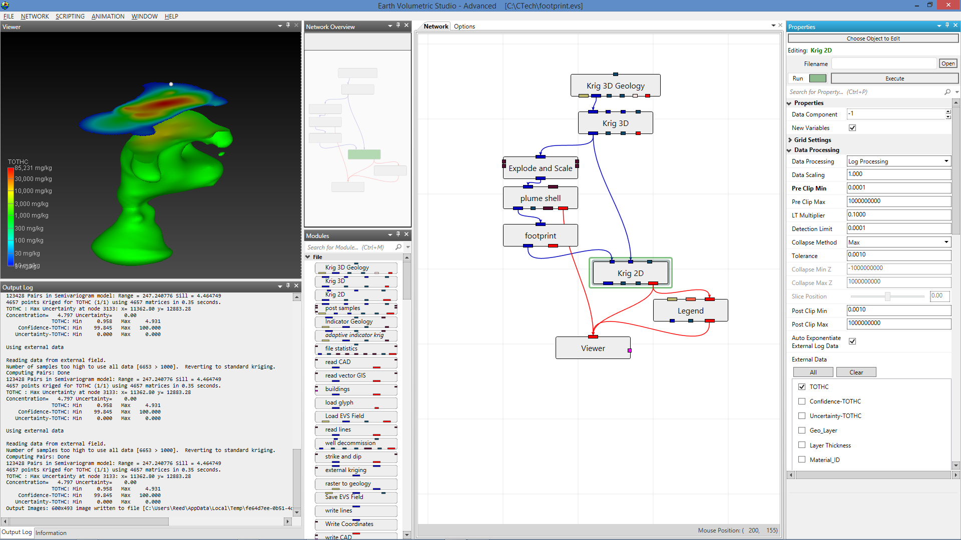
The footprint module is used to create the 2D footprint of a 3D input. It creates a surface at the specified Z Position with an x-y extent that matches the 3D input. The footprint output does not contain data, but data can be mapped onto it with external kriging.

NOTE: Do not use adaptive gridding when creating the 3D grid to be footprinted and mapping the maximum values with krig 2d (as in the example shown below). Footprint will produce the correct area, but krig 2d will map anomalous results when used with 3d estimation’s adaptive gridding.

Ports

Properties

Refinement

slope aspect splitter

The slope aspect splitter module will split an input field into two output fields based upon the slope and/or aspect of the external face of the cell and the subset expression used. The input field is split into two fields: one for which all cell orientations are true for the subset expression, and another field for which all cell orientations are false for the subset expression.

All data from the original input is preserved in the output.

Flat Surface Aspect: If you have a flat surface then a realistic aspect cannot be generated. This field lets you set the value for those cells.

1. To output all upward facing surfaces: use the default subset expression of SLOPE < 89.9. If your object was a perfect sphere, this would give you most of the upper hemisphere. Since the equator would be at slope of 90 degrees and the bottom would be >90 degrees.

(Notice there is potential for rounding errors, use 89.9 instead of 90)

Note: If your ground surface is perfectly flat and you wanted only it, you could use SLOPE < 0.01, however in the real world where topography exists, it can be difficult if not impossible to extract the ground surface and not get some other bits of surfaces that also meet your criteria.

2. General expression (assuming a standard cubic building):

A) SLOPE > 0.01 (Removes the top of the building)

B) SLOPE > 0.01 and SLOPE < 179.9 (Removes the top and bottom of the building)

3. Since ASPECT is a variable it must be defined for each cell. In cells with a slope of 0 or 180 there would be no aspect without our defining it with the flat surface aspect field.

4. Units are always degrees. You could change them to radians if you want inside the expression. (SLOPE * PI/180)

Ports

Properties

crop and downsize

The crop and downsize module is used to subset an image, or structured 1D, 2D or 3D mesh (an EVS “field” data type with implicit connectivity). Similar to cropping and resizing a photograph, crop and downsize sets ranges of cells in the I, J and K directions which create a subset of the data. When used on an image (which only has two dimensions), crop removes pixels along any of the four edges of the image. Additionally, crop and downsize reduces the resolution of the image or grid by an integer downsize value. If the resolution divided by this factor yields a remainder, these cells are dropped.

Crop and downsize refers to I, J, and K dimensions instead of x-y-z. This is done because grids are not required to be parallel to the coordinate axes, nor must the grid rows, columns and layers correspond to x, y, or z. You may have to experiment with this module to determine which coordinate axes or model faces are being cropped or downsized.

Ports

Properties

select cell sets

The select cell sets module provides the ability to select individual stratigraphic layers, lithologic materials or other cell sets for output. If connected to explode and scale, multiple select cell sets modules will allow selection of specific cell sets for downstream processing. One example would be to texture map the top layer with an aerial photo after one select cell sets and to color the other layers by data with a parallel select cell sets path. This can be accomplished by multiple explode and scale modules, but that would be much less efficient.

Ports

Properties

orthoslice

The orthoslice module is similar to the slice module, except limited to only displaying slice positions north-south (vertical), east-west (vertical) and horizontal. It subsets a structured field by extracting one slice plane and can only be orthogonal to the X, Y, or Z axis. Although less flexible in terms of capability, orthoslice is computationally more efficient.

Ports

Properties

edges

The edges module is similar to the external edges module in that it produces a wireframe representation of the nodal data making up an unstructured cell data mesh. There is however, no adjustment of edge angle and therefore only allows viewing of all grid boundaries (internal AND external) of the input mesh. The edges module is useful in that it is able to render lines around adaptive gridding locations whereas external edges does NOT render lines around this portion of the grid.

Ports

Properties

bounds

The bounds module generates lines and/or surfaces that indicate the bounding box of a 3D structured field. This is useful when you need to see the shape of an object and the structure of its mesh. This module is similar to external edges (set to edge angle = 60), except bounds allows for placing faces on the bounds of a model.

Bounds has one input port. Data passed to the port must contain any type of structured mesh (a grid definable with IJK resolution and no separable layers). Node Data can be present, but is only used if you switch on Data.

Ports

Properties