node_computation

The node_computation module is used to perform mathematical operations on nodal data fields and coordinates. Data values can be used to affect coordinates (x, y, or z) and coordinates can be used to affect data values.

Up to two fields can be input to node_computation. Mathematical expressions can involve one or both of the input fields**. Fields must be identical grids. This means they must have the same number of nodes and cells, otherwise the results will not make sense.**

Nodal data input to each of the ports is normally scalar, however if a vector data component is used, the values in the expression are automatically the magnitude of the vector (which is a scalar). If you want a particular component of a vector, insert an extract_scalar module before connecting a vector data component to node_computation. The output is always a scalar. If a data field contains more than one data component, you may select from any of them.

Module Input Ports

• Input Field 1[Field] Accepts a data field.
• Input Field 2[Field / minor] Accepts a data field.
• Input Value N1 [Number / minor] Accepts a number to be used in the field computations.
• Input Value N2 [Number / minor] Accepts a number to be used in the field computations.
• Input Value N3 [Number / minor] Accepts a number to be used in the field computations.
• Input Value N4 [Number / minor] Accepts a number to be used in the field computations.

Module Output Ports

• Output Field [Field] Outputs the subsetted field as faces.
• Output Value N1 [Number / minor] Outputs a number used in the field computations.
• Output Value N2 [Number / minor] Outputs a number used in the field computations.
• Output Value N3 [Number / minor] Outputs a number used in the field computations.
• Output Value N4 [Number / minor] Outputs a number used in the field computations.
• Output Object [Renderable]: Outputs to the viewer.

Module Parameters

• Data Definitions: You can have more than one new data component computed from each pass of node_computation. By default there is only Data0.
  • Add/Remove buttons allow you to add or remove Data Definitions
• Name: The data component name (e.g. Total Hydrocarbons)
• Units : The units of the data component (e.g. mg/kg)
• Log Process: When your input data is log processed, the values within node_computation will always be exponentiated.
  • In other words, even when your data is log processed, you will always see actual (not log) values.
  • This toggle should be ON whenever you are dealing with Log data.
  • If you want to perform math operations on the “Log” data, you must take the log of the An* or Bn* values within node_computation
  • If you do take the log of those values, you should always exponentiate the end results before exiting node_computation.

Each nodal data component from Input Field 1 is assigned as a variable to be used in the script. For example:

• An0 : First input data component
• An1 : Second input data component
• An2 : Third input data component
• An^N^ : Nth input data component

The min and max of these components are also added as variables :

• Min_An0 : Minimum of An0 data
• Max_An0 : Maximum of An0 data
• Min_An* : Minimum of An* data

For Input Field 2 the variable names change to:

• Bn0 : First input data component
• Bn1 : Second input data component
• Bn2 : Third input data component
• Bn^N^ : Nth input data component

An interesting and simple example of using node_computation can be found here.

The equation(s) used to modify data and/or coordinates must be input as part of a Python Script. The module will generate a default script and by modifying only one line (for the X coordinate)we get:

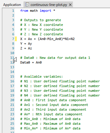
which with the following application:

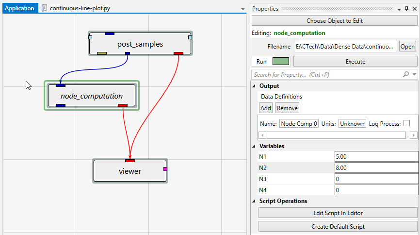
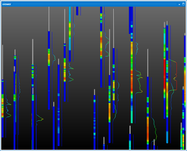
Gives us the ability to view densely sampled data as line plots beside each boring

cell_computation

The cell_computation module is used to perform mathematical operations on cell data in fields. Unlike node_compuation, it cannot affect coordinates.

Though data values can’t be used to affect coordinates (x, y, or z), the cell center (average of nodes) coordinates can be used to affect data values.

Up to two fields can be input to cell_computation. Mathematical expressions can involve one or both of the input fields.

Cell data input to each of the ports is scalar.

If a data field contains more than one data component, you may select from any of them.

Module Input Ports

• Input Field 1[Field] Accepts a data field.
• Input Field 2[Field / minor] Accepts a data field.
• Input Value N1 [Number / minor] Accepts a number to be used in the field computations.
• Input Value N2 [Number / minor] Accepts a number to be used in the field computations.
• Input Value N3 [Number / minor] Accepts a number to be used in the field computations.
• Input Value N4 [Number / minor] Accepts a number to be used in the field computations.

Module Output Ports

• Output Field [Field] Outputs the subsetted field as faces.
• Output Value N1 [Number / minor] Outputs a number used in the field computations.
• Output Value N2 [Number / minor] Outputs a number used in the field computations.
• Output Value N3 [Number / minor] Outputs a number used in the field computations.
• Output Value N4 [Number / minor] Outputs a number used in the field computations.
• Output Object [Renderable]: Outputs to the viewer.

Each cell data component from Input Field 1 is assigned as a variable to be used in the script. For example:

• An0 : First input data component
• An1 : Second input data component
• An2 : Third input data component
• An* : Nth input data component

The min and max of these components are also added as variables :

• Min_An0 : Minimum of An0 data
• Max_An0 : Maximum of An0 data
• Min_An* : Minimum of An* data

For Input Field 2 the variable names change to:

• Bn0 : First input data component
• Bn1 : Second input data component
• Bn2 : Third input data component
• Bn* : Nth input data component

combine_nodal_data

The combine_nodal_data module is used to create a new set of nodal data components by selecting components from up to six separate input data fields. The mesh (x-y-z coordinates) from the first input field, will be the mesh in the output. The input fields should have the same scale and origin, and number of nodes in order for the output data to have any meaning. This module is useful for combining data contained in multiple field ports or files, or from different Kriging modules.

Module Input Ports

• Model Field [Field] Accepts a field with data whose grid will be exported.
• Input Field 1 [Field] Accepts a data field.
• Input Field 2 [Field] Accepts a data field.
• Input Field 3 [Field] Accepts a data field.
• Input Field 4 [Field] Accepts a data field.
• Input Field 5 [Field] Accepts a data field.

Module Output Ports

• Output Field [Field] Outputs the field with selected data
• Output Object [Renderable]: Outputs to the viewer.

interpolate data

The interpolate data module interpolates nodal and/or cell data from a 3D or 2D field to either a 2D mesh or 1D line. Typical uses of this module are mapping of data from a 3D mesh onto a geologic surface or a 2D fence section. In these applications the 2D surface(s) simply provide the new geometry (mesh) onto which the adjacent nodal values are interpolated. The primary requirement is that the data be equal or higher dimensionality than the mesh to be interpolated onto. For instance, if the user has a 2D surface with nodal data (perhaps z values), then a 1D line may be input and the nearest nodal values from the 2D surface will be interpolated onto it.

NOTE: This module supplants interpolate nodal data and interpolate cell data.

Module Input Ports

• Input Data Field [Field] Accepts a data field.
• Input Destination Field [Field] Accepts a field onto which the data will be interpolated

Module Output Ports

• Output Field [Field] Outputs the field Destination Field with new data
• Output Object [Renderable]: Outputs to the viewer.

The compute thickness module allows you to compute the thickness of complex plumes or cell sets such as lithologic modeling’s materials.

Module Input Ports

• Input Field The field to map thickness data onto
• Input Volume The (volumetric) field to determine thickness data from

Module Output Ports

• Output Field The surface (or 3D object) with mapped thickness data

Important Features and Considerations

The right input port must have a 3D field as input.

• There is no concept of thickness associated with 2D or 3D surfaces
• Volumetric inputs can be plume_shell or intersection_shell objects which are hollow.
  • Thickness will be determined based upon the apparent thickness of the plume elements.
  • When 3D Shells are input, they must be closed objects.

Determining thickness of arbitrary volumetric objects is a very computationally intensive operation. You can use this module to compute thickness in two primary ways:

• Compute the thickness distribution of a 3D object and project that onto a 2D surface (generally at the ground surface)
  • A surface (such as from geologic surface) would connect to the first (left) input port
  • The volumetric object connects to the second (right) input port
• Compute the thickness distribution of a 3D object and project that onto the same object
  • The volumetric object connects to the first (left) input port
  • The same volumetric object connects to the second (right) input port

Note: In all cases run times can be long. Coarser grids and the first option will run faster, but the complexity and resolution of the volumetric object will be the major factor in the computation time.

translate by data

The translate by data module accepts nearly any mesh and translates the grid in x, y, or z based upon either a nodal or cell data component or a constant.

The interface enables changing the Scale Factor for z translates to accommodate an overall z exaggeration in your applications. This module is most useful when used with the import vector gis module to properly place polygonal shapefile cells at the proper elevation.

Warning: The scale factor is always applied. If translating along any axis other than z, it is unlikely that you want to use the Z Exaggeration factor used elsewhere in your application.

• When translating by a Constant, the amount is affected by the Z Scale Factor.
• When translating by Cell Data, a radio box appears to allow specification of the cell data component
• When translating by Node Data, a radio box appears to allow specification of the nodal data component

Module Input Ports

• Z Scale [Number] Accepts Z Scale (vertical exaggeration).
• Input Field [Field] Accepts a data field from 3d estimation or other similar modules.

Module Output Ports

• Z Scale [Number] Outputs Z Scale (vertical exaggeration) to other modules
• Output Field [Field] Outputs the subsetted field
• Scale Link
• Output Object [Renderable]: Outputs to the viewer

cell data to node data

The cell data to node data module is used to translate cell data components to nodal data components. Cell data components are data components which are associated with cells rather than nodes. Most modules in EVS that deal with analytical or continuum data support node based data. Therefore, cell data to node data can be used to translate cell based data to a nodal data structure consistent with other EVS modules.

Module Input Ports

• Input Field [Field] Accepts a field with cell data.

Module Output Ports

• Output Field [Field / Minor] Outputs the field with cell data converted to nodal data
• Output Object [Renderable]: Outputs to the viewer.

The node data to cell data module is used to translate nodal data components to cell data components. Cell data components are data components which are associated with cells rather than nodes. Most modules in EVS that deal with analytical or continuum data support node based data, and those that deal with geology (lithology) tend to use cell data. Therefore, node data to cell data can be used to translate nodal data to cell data.

Module Input Ports

• Input Field [Field] Accepts a field with nodal data.

Module Output Ports

• Output Field [Field / Minor] Outputs the field with nodal data converted to cell data
• Output Object [Renderable]: Outputs to the viewer.

shrink cells

The shrink cells module produces a mesh containing disjoint cells which can be optionally shrunk relative to their geometric centers. It creates duplicate nodes for all cells that share the same node, making them disjoint. If the shrink cells toggle is set, the module computes new coordinates for the nodes based on the specified shrink factor (which specifies the scale relative to the geometric centers of each cell). The shrink factor can vary from 0 to 1. A value of 0 produces non-shrunk cells; 1 produces completely collapsed cells (points). This module is useful for separate viewing of cells comprising a mesh.

Module Input Ports

• Input Field [Field] Accepts a field

Module Output Ports

• Output Field [Field / Minor] Outputs the field with modified cells
• Output Object [Renderable]: Outputs to the viewer

cell centers

cell centers module produces a mesh containing Point cell set, each point of which represents a geometrical center of a corresponding cell in the input mesh. The coordinates of cell centers are calculated by averaging coordinates of all the nodes of a cell. The number of nodes in the output mesh is equal to number of cells in the input mesh. If the input mesh contains Cell_Data it becomes a Node_Data in the output mesh with each node values equal to corresponding cell value. Nodal data is not output directly. You can use this module to create a position mesh for the glyphs at nodes module. You may also use this module as mesh input to the interpolate data module, then send the same nodal values as the input grid, to create interpolated nodal values at cell centroids.

Module Input Ports

• Input Field [Field] Accepts a field.

Module Output Ports

• Output Field [Field / Minor] Outputs the field as points representing the centers of the cells.
• Output Object [Renderable]: Outputs to the viewer.

This module allows you to assign data and subset all (or selected) discrete (disconnected) regions of plumes or lithologic materials.

• OVERVIEW: When we create subsets of models, either based upon analytical data, stratigraphic or lithologic modeling these subsets often exist as several disjoint pieces.

  • In the case of analytical (e.g., contaminant) plumes, the number and size of regions (pieces) can strongly depend on the subsetting level.
  • With lithologic models, the number and size of the regions depends on the complexity of the lithologic data and the modeling parameters.

• FUNCTION: The connectivity assessment module assigns a new data component to these dis-connected regions.

  • The pieces are sorted based upon the number of cells in each piece.

    • This is generally well correlated to the volume of that regions, but it is definitely possible that the region with the most cells may not have the greatest volume.

  • The highest cell count region is assigned to 0 (zero) and regions with descending cell counts are assigned higher integer values.

• PARAMETERS:

  1. Merge Cell Sets (toggle): Merges cell sets such as stratigraphic layers or lithologic materials. Generally should be on when dealing with analytical data.

  2. Assessment Mode: Determines the criteria for subsetting of regions and/or assigning data

     1. Add Region ID Data: Does not subset, but assigns Cell Data corresponding to cell counts
     2. Subset By Region ID(s)
     3. Region Closest to Point
     4. Region with most cells: Outputs Region ID = 0 without assigning data.

  3. Point Coordinate: Is the X, Y, Z coordinate to be used for “Closest region”

  4. Region IDs: The list of regions to include in the output if Selection Mode is set to “Subset By Region ID”