Module Libraries
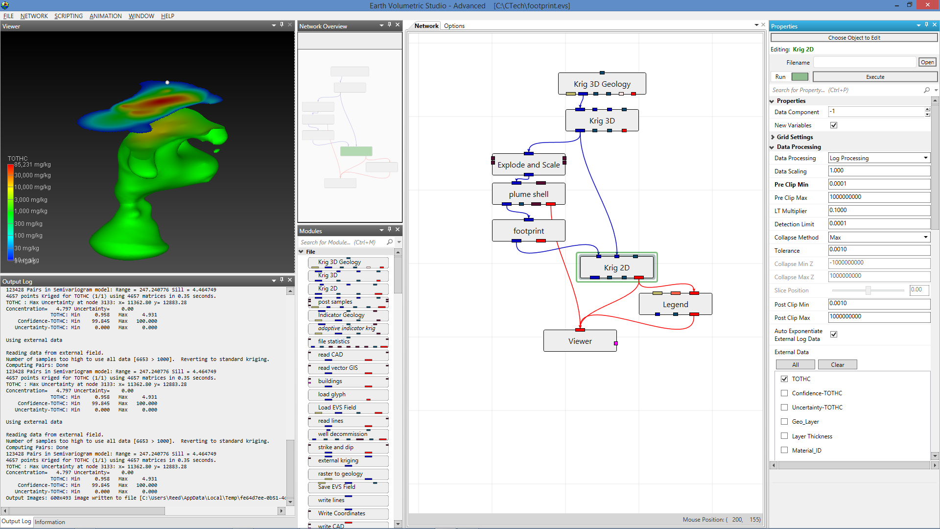
EVS modules can each be considered software applications that can be combined together by the user to form high level customized applications performing analysis and visualization. These modules have input and output ports and user interfaces.
The library of module are grouped into the following categories:
- Estimation modules take sparse data and map it to surface and volumetric grids
- Geology modules provide methods to create surfaces or 3D volumetric grids with lithology and stratigraphy assigned to groups of cells
- Display modules are focused on visualization functions
- Analysis modules provide quantification and statistical information
- Annotation modules allow you to add axes, titles and other references to your visualizations
- Subsetting modules extract a subset of your grids or data in order to perform boolean operations
- Proximity modules create new data which can be used to subset or assess proximity to surfaces, areas or lines.
- Processing modules act on your data
- Import modules read files that contain grids, data and/or archives
- Export modules write files that grids, data and/or archives
- Modeling modules are focused on functionality related to simulations and vector data
- Geometry modules create or act upon grids and geometric primitives
- Projection modules transform grids into other coordinates or dimensionality
- Image modules are focused on aerial photos or bitmap operations
- Time modules provide the ability to deal with time domain data
- Tools are a collection of modules to make life easier
- View modules are focused on visualization and output of results
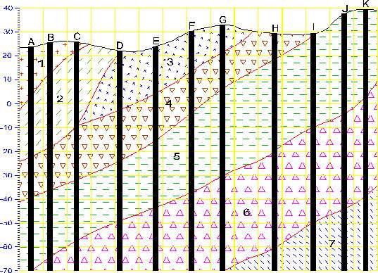
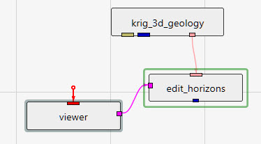
Revisions to Module Names Effective After EVS Version 2021.10 Effective October 2021, there was a major revision to module naming. The table below lists the old and new names. Also note that the Cell Data library was eliminated with its modules moved to Processing. In general the new module names are intended to be more descriptive of each module’s functionality. For example, krig_3d_geology was named over 25 years ago when we developed it to create 3D stratigraphic models using kriging to estimate the horizons. It now does not use kriging as its default estimation method (of many) and is often used to build grids that are solely conformal to surface topography. Its new name “gridding and horizons” is far more descriptive of its current use.
3d estimation 3d estimation 3d estimation performs parameter estimation using kriging and other methods to map 3D analytical data onto volumetric grids defined by the limits of the data set, or by the convex hull, rectilinear, or finite-difference grid extents of a geologic system modeled by gridding and horizons. 3d estimation provides several convenient options for pre- and post-processing the input parameter values, and allows the user to consider anisotropy in the medium containing the property.
create stratigraphic hierarchy create stratigraphic hierarchy The create stratigraphic hierarchy module reads a special input file format called a pgf file, and then allows the user to build geologic surfaces based on the input file’s geologic surface intersections. This process is carried out visually (in the EVS viewer) with the use of the create stratigraphic hierarchy user interface. The surface hierarchy can either be generated automatically for simple geology models or for every layer for complex models. When the user is finished creating surfaces the gmf file can be finalized and converted into a *.GEO file.
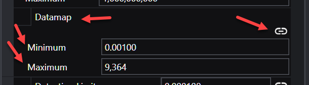
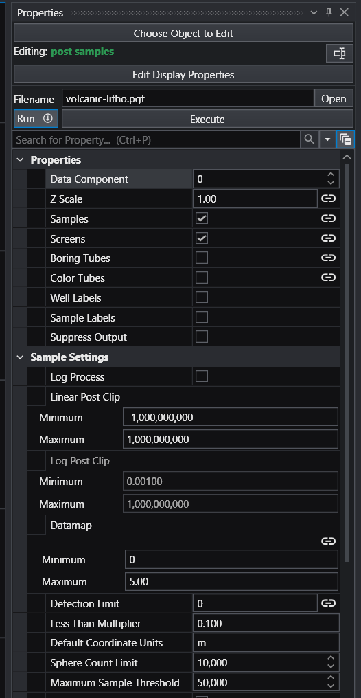
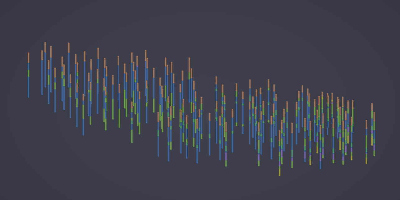
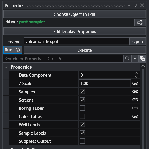
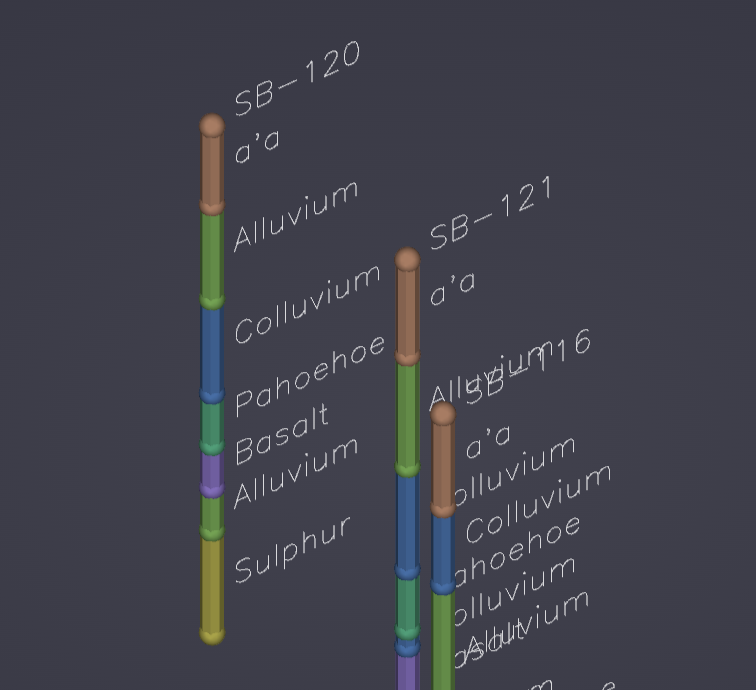
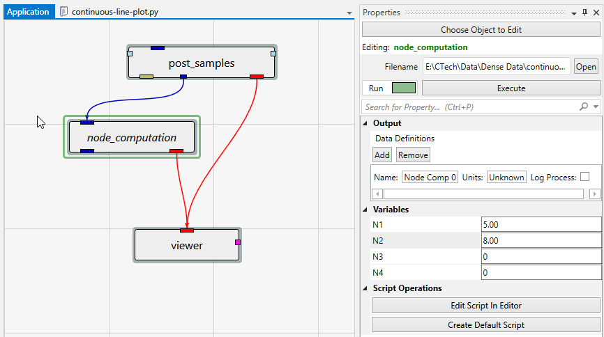
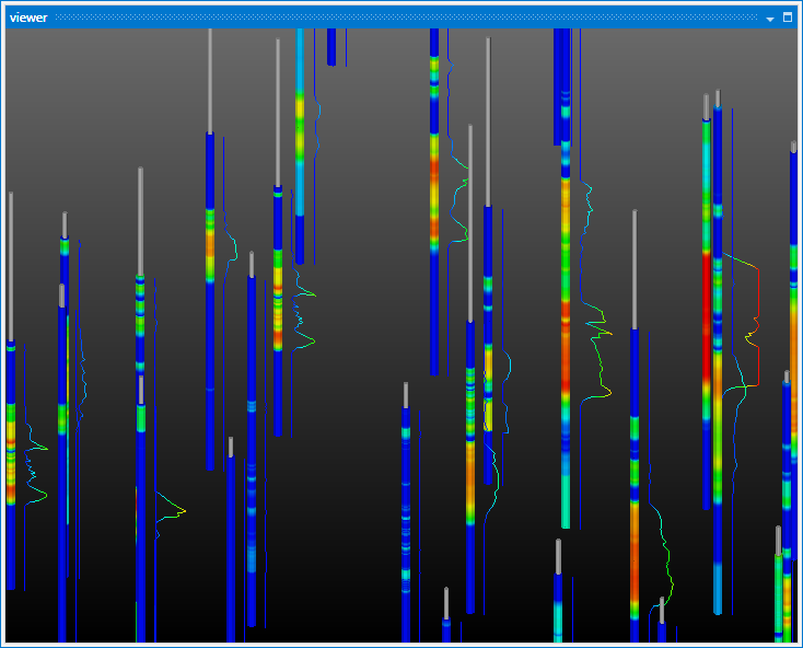
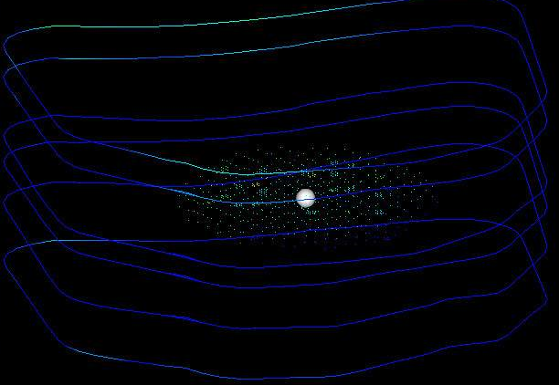
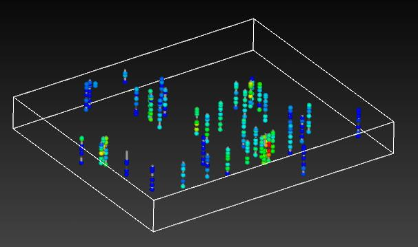
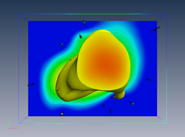
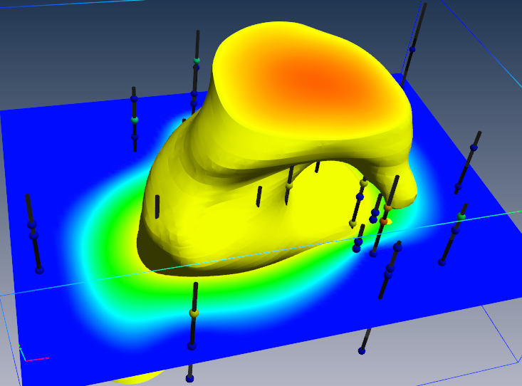
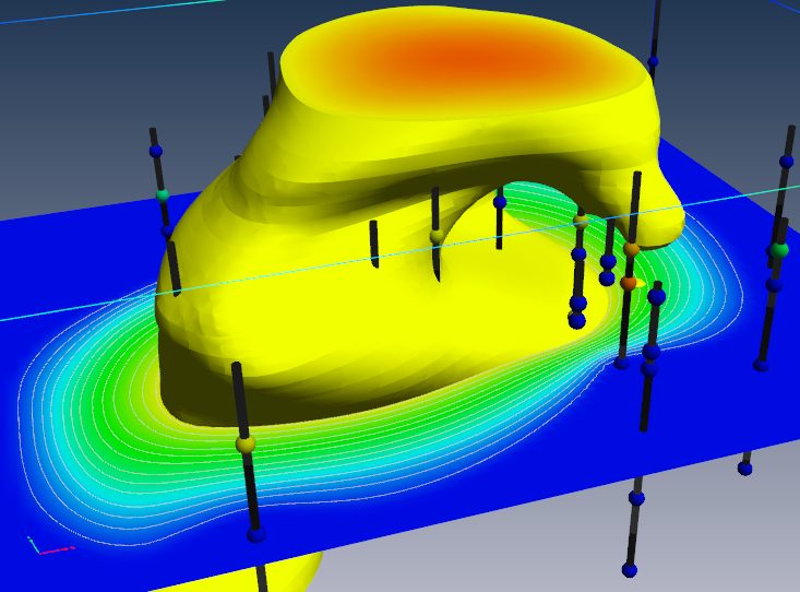
post samples post_samples The post_samples module is used to visualize: Sampling locations and the values of the properties in .apdv files The lithology specified in a .pgf, .lsdv, .lpdv or .geo files The location and values of well screens in a .aidv file Warning When using the Datamap parameters (Minimum and Maximum) unlinked such the the resulting datamap is a subset of the true data range, probing in C Tech Web Scenes will only be able to report values within the truncated data range. Values outside that limited range will display the nearest value within the truncated range.
volumetrics volumetrics The volumetrics module is used to calculate the volumes and masses of soil, and chemicals in soils and ground water, within a user specified constant_shell (surface of constant concentration), and set of geologic layers. The user inputs the units for the nodal properties, model coordinates, and the type of processing that has been applied to the nodal data values, specifies the subsetting level and soil and chemical properties to be used in the calculation, and the module performs an integration of both the soil volumes and chemical masses that are within the specified constant_shell. The results of the integration are displayed in the EVS Information Window, and in the module output window.
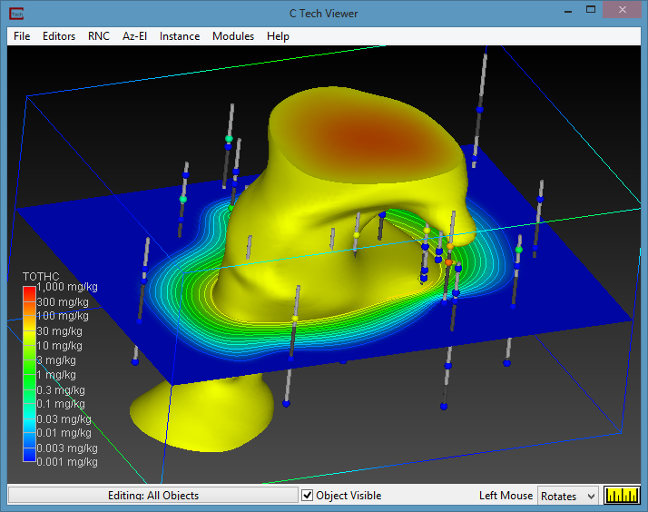
legend legend The legend module is used to place a legend which help correlate colors to analytical values or materials . The legend shows the relationship between the selected data component for a particular module and the colors shown in the viewer. For this reason, the legend’s RED input port must be connected to the RED output port of a module which is connected to the viewer and is generally the dominant colored object in view.
external faces external_faces The external_faces module extracts external faces from a 2D or 3D field for rendering. external_faces produces a mesh of only the external faces of each cell set of a data set. Because each cell set’s external faces are created there may be faces that are seemingly internal (vs. external). This is especially true when external faces is used subsequent to a plume module on 3D (volumetric) input.
distance to 2d area distance to 2d area distance to 2d area receives any 3D field into its left input port and it receives triangulated polygons (from triangulate_polygon, or other sources) into its right input port. Its function is similar to buffer distance or distance to shape. It adds a data component to the input 3D field and using plume_shell, you can cut structures inside or outside of the input polygons. Only the x and y coordinates of the polygons are used because distance to 2d area cuts a projected slice that is z invariant. distance to 2d area recalculates when either input field is changed or the “Accept” button is pressed.
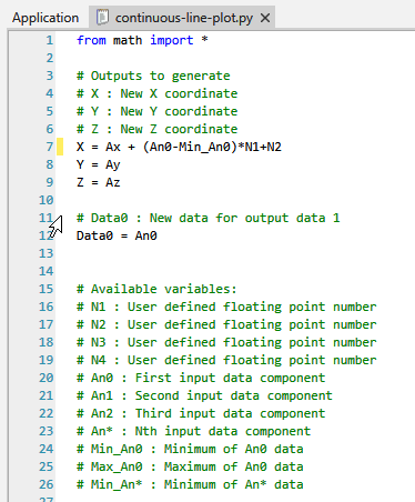
node computation node_computation The node_computation module is used to perform mathematical operations on nodal data fields and coordinates. Data values can be used to affect coordinates (x, y, or z) and coordinates can be used to affect data values. Up to two fields can be input to node_computation. Mathematical expressions can involve one or both of the input fields**. Fields must be identical grids. This means they must have the same number of nodes and cells, otherwise the results will not make sense.**
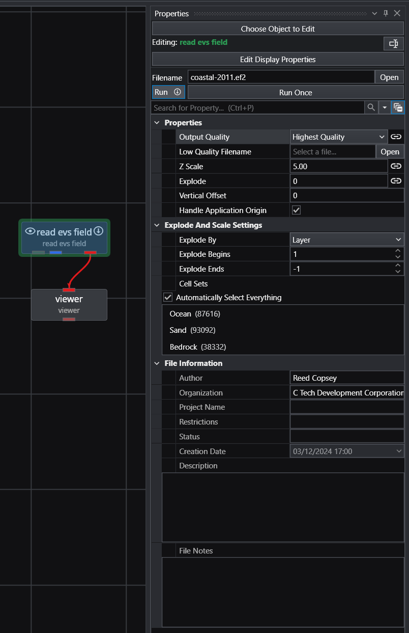
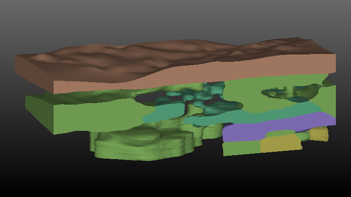
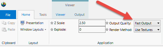
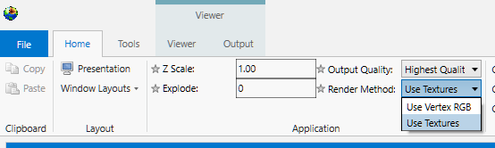
read evs field read evs field read evs field reads a dataset from the primary and legacy file formats created by write evs field. .EF2: The only Lossless format for models created in 2024 and later versions .eff ASCII format, best if you want to be able to open the file in an editor or print it. For a description of the .EFF file formats click here. .efz GNU Zip compressed ASCII, same as .eff but in a zip archive .efb binary compressed format, the smallest & fastest format due to its binary form Output Quality: An important feature of read evs field is the ability to specify two separate files which correspond to High Quality (e.g. fine grids) and Low Quality (e.g. coarse grids a.k.a. fast).
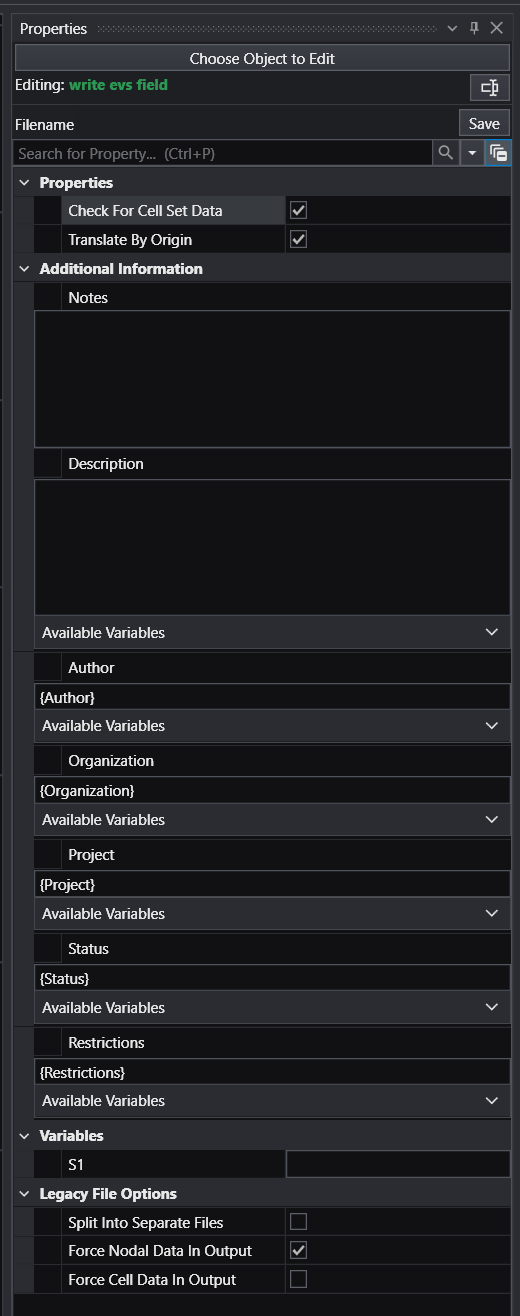
write evs field write evs field The write evs field module creates a file in one of several formats containing the mesh and nodal and/or cell data component information sent to the input port. This module is useful for writing the output of modules which manipulate or interpolate data (3d estimation , 2d estimation, etc.) so that the data will not need to be processed in the future.
driven sequence The driven sequence module controls the semi-automatic creation of sequences for the following modules: scripted sequence The scripted sequence module provides the most power and flexibility, but requires creating a Python script which sets the states of all modules to be object sequence This is the simplest of the sequence modules, but also the easiest to abuse (vs. using scripted sequence where you can be more efficient).
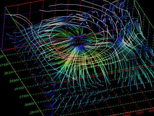
3d streamlines 3d streamlines The 3d streamlines module is used to produce streamlines or stream-ribbons of a field which is a 2 or 3 element vector data component on any type of mesh. Streamlines, which are simply 3D polylines, represent the pathways particles would travel based on the gradient of the vector field. At least one of the nodal data components input to streamlines must be a vector. The direction of travel of streamlines can be specified to be forwards (toward high vector magnitudes) or backwards (toward low vector magnitudes) with respect to the vector field. Streamlines are produced by integrating a velocity field using the Runge-Kutte method of specified order with adaptive time steps.
draw lines draw_lines The draw_lines module enables you to create both 2D and 3D lines interactively with the mouse. The mouse gesture for line creation is: depress the Ctrl key and then click the left mouse button on any pickable object in the viewer. The first click establishes the beginning point of the line segment and the second click establishes each successive point. polyline processing polyline processing The polyline processing module accepts a 3D polyline and can either increase or decrease the number of line segments of the polyline. A splining algorithm smooths the line trajectory once the number of points are specified. This module is useful for applications such as a fly over application (along a polyline path drawn by the user). If the user drawn line is jagged with erratically spaced line segments, polyline spline smooths the path and creates evenly spaced line segments along the path.
project onto surface project onto surface project onto surface provides a mechanism to drape lines and triangles (surfaces) onto surfaces. Please note that a pseudo-3D object like a building made up of triangle faces will be flattened onto the surface. The 3D nature will not be preserved. Lines and surfaces are subsetted to match the size of the cells of the surface on which the lines are draped. In other words, draped objects will match the surface precisely.
overlay aerial overlay_aerial The overlay_aerial module will take as input a field and then map an image onto the horizontal areas of the grid. The image can be projected from one coordinate system to another. It can also be georeferenced if it has an accompanying All vertical surfaces (Walls) can be included in the output but will not have image data mapped to them. texture cross section texture_cross_section allows you to apply images along a complex non-linear cross section (cross-section) path and compensate for the image scale an
read tcf read_tcf The read_tcf module is specifically designed to create models and animations of data that changes over time. This type of data can result from water table elevation and/or chemical measurements taken at discrete times or output from Groundwater simulations or other 3D time-domain simulations. The read_tcf module creates a field using a Time Control File (.TCF) to specify the date/time, field and corresponding data component to read (in netCDF, Field or UCD format), for each time step of a time_data field. All file types specified in the TCF file must be the same (e.g. all netCDF or all UCD). The same file can be repeated, specifying different data components to represent different time steps of the output.
group objects group objects group objects is a renderable object that contains other subobjects that have the attributes that control how the rendering is done. Unlike DataObject, group objects does not include data. Instead, it is meant to be a node in the rendering hierarchy that groups other DataObjects together and supplies common attributes from them. This object is connected directly to one of the viewers (for example, Simpleviewer3D) or to another DataObject or to group objects. A group objects is included in all the standard viewers provided with the EVS applications chooses.
viewer viewer The viewer accepts renderable objects from all modules with red output ports to include their output in the view. Module Input Ports Objects [Renderable]: Receives renderable objects from any number of modules Module Output Ports View [View / minor] Outputs the view information used by other modules to provide all model extents or interactivity viewer Properties: The user interfaces for the viewer are arranged in 10 categories which cover interaction with the scene, the characteristics of the viewer as well as various output options.
scat_to_unif scat_to_unif The scat_to_unif module is used to convert scattered sample data into a three-dimensional uniform field. Also, scat_to_unif can be used to take an existing grid (for example a UCD file) and convert it to a uniform field. scat_to_unif converts a field of non-uniformly spaced points into a uniform field which can be used with many of EVS’s filter and mapper modules. “Scattered sample data " means that there are disconnected nodes in space. An example would be geology or analyte (e.g. chemistry) data where the coordinates are the x, y, and elevation of a measured parameter. The data is “scattered” because there isn’t data for every x/y/elevation of interest.