read evs field read evs field reads a dataset from the primary and legacy file formats created by write evs field. .EF2: The only Lossless format for models created in 2024 and later versions .eff ASCII format, best if you want to be able to open the file in an editor or print it. For a description of the .EFF file formats click here. .efz GNU Zip compressed ASCII, same as .eff but in a zip archive .efb binary compressed format, the smallest & fastest format due to its binary form Output Quality: An important feature of read evs field is the ability to specify two separate files which correspond to High Quality (e.g. fine grids) and Low Quality (e.g. coarse grids a.k.a. fast).
import vtk import vtk reads a dataset from any of the following 9 VTK file formats. Please note that VTK’s file formats do not include coordinate units information, not analyte units. There is a parameter which allows you to specify coordinate units (meters are the default). vtk: legacy format vtr: Rectilinear grids vtp: Polygons (surfaces) vts: Structured grids vtu: Unstructured grids pvtp: Partitioned Polygons (surfaces) pvtr: Partitioned Rectilinear grids pvts: Partitioned Structured grids pvtu: Partitioned Unstructured grids Module Output Ports
import cad General Module Function The import cad module will read the following versions of CAD files: AutoCAD DWG and DXF files through AutoCAD 2021 (version 24.0) Bentley Microstation DGN files through Version 8. This module provides the user with the capability to integrate site plans, buildings, and other 2D or 3D features into the EVS visualization, to provide a frame of reference for understanding the three dimensional relationships between the site features, and characteristics of geologic, hydrologic, and chemical features. The drawing entities are treated as three dimensional objects, which provides the user with a lot of flexibility in the placement of CAD objects in relation to EVS objects in the visualization. The project onto surface and geologic_surfmap modules allow the user to drape CAD line-type entities (not 3D-Faces) onto three dimensional surfaces.
import vector gis The import vector gis module reads the following vector file formats: ESRI Shapefile (.shp); Arc/Info E00 (ASCII) Coverage (.e00); Atlas BNA file (.bna); GeoConcept text export (.gxt); GMT ASCII Vectors (.gmt); and the MapInfo TAB (.tab) format. Module Input Ports Z Scale [Number] Accepts Z Scale (vertical exaggeration) from other modules Module Output Ports Z Scale [Number] Outputs Z Scale (vertical exaggeration) to other modules Output [Field] Outputs the GIS data. Output Object [Renderable]: Outputs to the viewer Properties and Parameters
import raster as horizon The import raster as horizon module reads several different raster format files in EVS Geology format. These formats include DEMs, Surfer grid files, Mr. Sid files, ADF files, etc.. Multiple import raster as horizon modules can be combined with combine horizons into a 3D geologic model. Alternatively, a single file can be displayed as a surface (with surfaces from horizons) or you can export its coordinates (with export nodes) to use the values in a GMF file.
buildings The buildings module reads C Tech’s .BLDG file and creates various 3D objects (boxes, cylinders, wedge-shapes for roofs, simple houses etc.), and provides a means for scaling the objects and/or placing the objects at user specified locations. The objects are displayed based on x, y & z coordinates supplied by the user in a .bldg file, with additional scaling option controls on the buildings user interface.
read_lines The read_lines module is used to visualize a series of points with data connected by lines. read_lines accepts three different file formats, with the APDV file format the lines are connected by boring ID, with the ELF (EVS Line File) format each line is made by defining the points that make up the line, and with the SAD (Strike and Dip) file format, there is a choice to connect each sample by ID or by Data Value.
read strike and dip General Module Function The read strike and dip module is used to visualize sampled locations. It places a disk, oriented by strike and dip, at each sample location. Each disk is probable and can be colored by a picked color, by Id, or by data value. If an ID is present, such as a boring ID, then there is an option to place tubes between connected disks, or those disks with similar Id’s.
read glyph read glyph replaces the Glyphs sub-library that was in the tools library. It reads glyphs saved in any of the three primary EVS field file formats and allows you to modify the shape and orientation of the glyph to allow it to be used in various modules that emply glyphs in slightly different ways. These include glyphs at nodes, place_glyph,drive_glyphs, advector, post_samples, etc. Most modules EXCEPT post_samples will use the glyphs without chaning the default alignment. The supported file formats are:
General Module Function
Subsections of Import
read evs field
read evs field reads a dataset from the primary and legacy file formats created by write evs field.
- .EF2: The only Lossless format for models created in 2024 and later versions
- .eff ASCII format, best if you want to be able to open the file in an editor or print it. For a description of the .EFF file formats click here.
- .efz GNU Zip compressed ASCII, same as .eff but in a zip archive
- .efb binary compressed format, the smallest & fastest format due to its binary form
Output Quality: An important feature of read evs field is the ability to specify two separate files which correspond to High Quality (e.g. fine grids) and Low Quality (e.g. coarse grids a.k.a. fast).
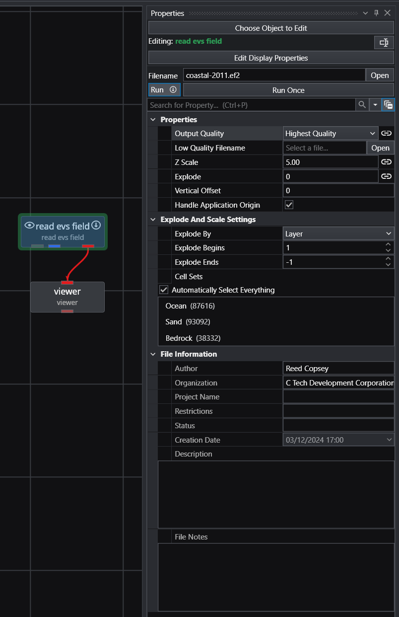
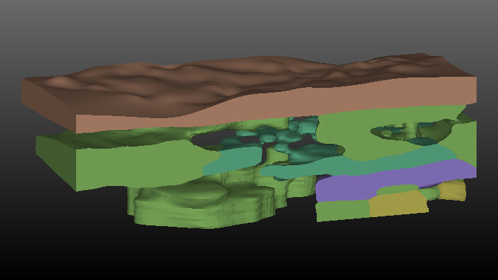
You can see that read evs field is specifying two different EFB files. The Output Quality is set to Highest Quality and is Linked (black circle). The viewer shows:
If we change the Output Quality on the Home Tab
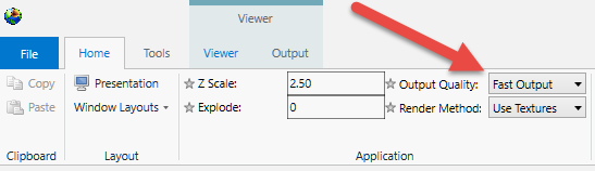
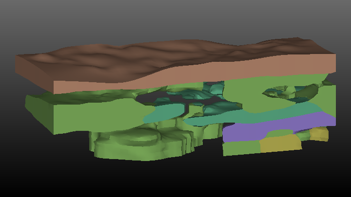
It changes the setting in read evs field and the viewer changes to show:
Though you “can” change the Output Quality in read evs field, it is best to change it on the Home Tab to make sure that all read evs field modules in your application will have the same setting. This is not relevant to this simple application, but if we were using a cutting surface (saved as fine and coarse EFBs) and doing distance to surface operations on a very large grid, this synchronization would be important.
read evs field effectively has explode_and_scale and an external_faces module built in. This allows the module to perform:
- Z Scaling
- Exploding
- Nodal or Cell data selection
- Selection of cell_sets
Module Output Ports
- Geologic legend Information [Geology legend] Supplies the geologic material information for the legend module.
- Output [Field] Outputs the saved field.
- File Notes [String / minor] Outputs a string to document the settings used to create the field.
- Output Object [Renderable]: Outputs to the viewer.
EVS Field File Formats and Examples EVS Field file formats supplant the need for UCD, netCDF, Field (.fld), EVS_Geology by incorporating all of their functionality and more in a new file format with three mode options. .eff ASCII format, best if you want to be able to open the file in an editor or print it
Subsections of read evs field
EVS Field File Formats and Examples
EVS Field file formats supplant the need for UCD, netCDF, Field (.fld), EVS_Geology by incorporating all of their functionality and more in a new file format with three mode options.
.eff ASCII format, best if you want to be able to open the file in an editor or print it
.efz GNU Zip compressed ASCII, same as .eff but in a zip archive
.efb binary compressed format, the smallest & fastest format due to its binary form
Here are the tags available in an EVS field file, in the appropriate order. Note that no file will contain ALL these tags, as some are specific to the type of field (based on definition). The binary file format is undocumented and exclusively used by C Tech’s write evs field module.
If the file is written compressed, the .efz file (and any split, extra data files) will all be compressed. The compression algorithm is compatible with the free gzip/gunzip programs or WinZip, so the user can uncompress a .efz file and get an .eff file at will. The .efb file is also compressed (hence its very small size), but uncompressing this file will not make it human-readable.
EVS Field Files
EVS Field Files consist of file tags that delineate the various sections of the file(s) and data (coordinates, nodal and/or cell data, and connectivity). The file tags are discussed below followed by portions of a few example files.
FILE TAGS:
The file tags for the ASCII file formats (shown in Bold Italics) are discussed below with a representative example. They are given in the appropriate order. If you need assistance creating software to write these file formats, please contact support@ctech.com.
DATE_CREATED(optional) 7/16/2004 1:57:55 PM
The creation date of the file.
EVS_FIELD_FILE_NOTES_START (optional)
Insert your Field file notes here.
EVS_FIELD_FILE_NOTES_END
This is the file description block. These notes are used to describe the contents of the Field file. The entire block is optional, however if you wish to use notes then both the starting and end tag are required.
DEFINITION Mesh+Node_Data
This is the type of field we are creating. Typically options are:
Mesh+Node_Data
Mesh+Cell_Data
Mesh+Node_Data+Cell_Data
Mesh_Struct+Node_Data (Geology)
Mesh_Unif+Node_Data (Uniform field)
NSPACE 3
nspace of the output field. Typically 3, but 2 in the case of geology or an image
NNODES 66355
Number of nodes. Not used for Mesh_Struct of Mesh_Unif
NDIM 2
Number of dimensions in a Mesh_Struct or Mesh_Unif
DIMS 41 41
The dimensions for a mesh_struct or uniform field
POINTS 11061.528999 12692.304504 -44.049999 11611.330994 13098.105469 11.500000
The lower left and upper right corner of a uniform field (Mesh_Unif only)
COORD_UNITS “ft”
Coordinate Units
NUM_NODE_DATA 7
Number of nodal data components
NUM_CELL_DATA 1
Number of cell data components
NCELL_SETS 5
Number of cell sets
NODES FILE “test_split.xyz” ROW 1 X 1 Y 2 Z 3
Nodes section is starting. If it says “NODES IN_FILE”, the nodes follow (x/y/z) on the next nnodes rows, otherwise, the line will say FILE “filename” ROW 1 X 1 Y 2 Z 3, which is the file to get the coordinates, the row to start at (1 is first line of file), and the columns containing your X, Y, and Z values
NODE_DATA_DEF 0 “TOTHC” “log_ppm” MINMAX -3 4.592 FILE “test_split.nd” ROW 1 COLS 1
NODE_DATA_DEF specifies the definition of a nodal data component. The second word is the data component number, the third is the name, the 4th is the units, then it will either say IN_FILE (which means that it will start after a NODE_DATA_START tag) or the file information. Other options are:
MINMAX - two numbers follow which are the data minimum and maximum. This behaves much like the set_min_max module.
If this is vector data, there will be a VECLEN 3 tag in there, and COLS will need to have 3 numbers following it (for each component of the vector)
NODE_DATA_START. All the node data components that are specified IN_FILE are listed in order after this tag.
CELL_SET_DEF 0 8120 Hex “Fill” MINMAX 1 14 FILE “test_split.conn” ROW 1
Definition of a cell set. 2nd word is cell set number, 3rd is number of cells, 4th is type, 5th is the name, then its either IN_FILE (which means they will be listed in order by cell set), or the FILE “filename” section and a row to begin reading from. Other options are:
MINMAX - two numbers follow which are the data minimum and maximum. This behaves much like the cell_set_min_max module.
CELL_START. Start of all the cell set definitions that are specified IN_FILE.
CELL_DATA_DEF 0 “Indicator” “Discreet Unit” FILE “test_split.cd” ROW 1 COLS 1
Definition of cell data. Same options as NODE_DATA_DEF
CELL_DATA_START
Start of all cell data that is specified as IN_FILE
LAYER_NAMES “Top” “Fill” “Silt” “Clay” “Gravel” “Sand”
Allows you to specify the names associated with surfaces (layers)
MATERIAL_MAPPING “1|Silt” “2|Fill” “3|Clay” “4|Sand” “5|Gravel”
Allows you to specify the Material_ID and the associated material names. Note that each number/name pair is in quotes, with the name separated from the number by the pipe “|” symbol.
END
Marks the end of the data section of the file. (Allows us to put a password on .eff files)
EVS Field File Examples:
Because EVS Field Files can contain so many different types of grids, it is beyond the scope of our help system to include every variant.
3d estimation - EFF file representing a uniform field: The file below is an abbreviated example of writing the output of 3d estimation having kriged a uniform field (which can be volume rendered). Large sections of the data regions of this file are omitted to save space. This is represented by sections of the file with “*** omitted ***” replacing many lines of data.
DEFINITION Mesh_Unif+Node_Data
NSPACE 3
NDIM 3
DIMS 41 41 35
COORD_UNITS “ft”
NUM_NODE_DATA 7
POINTS 11281.910004 12211.149994 -29.900000 12515.890015 13259.449951 0.900000
NODE_DATA_DEF 0 “VOC” “log_ppm” IN_FILE
NODE_DATA_DEF 1 “Confidence-VOC” “linear_%” IN_FILE
NODE_DATA_DEF 2 “Uncertainty-VOC” “linear_Unc” IN_FILE
NODE_DATA_DEF 3 “Geo_Layer” “linear_” IN_FILE
NODE_DATA_DEF 4 “Elevation” “linear_ft” IN_FILE
NODE_DATA_DEF 5 “Layer Thickness” “linear_ft” IN_FILE
NODE_DATA_DEF 6 “Material_ID” “linear_” IN_FILE
NODE_DATA_START
-2.357487 34.455845 2.325005 0.000000 -29.900000 30.799999 0.000000
-3.000000 34.977974 0.000000 0.000000 -29.900000 30.799999 0.000000
-3.000000 35.603794 0.000000 0.000000 -29.900000 30.799999 0.000000
***** OMITTED *****
-3.000000 30.056839 0.000000 0.000000 0.900000 30.799999 0.000000
-3.000000 29.858747 0.000000 0.000000 0.900000 30.799999 0.000000
-3.000000 29.673925 0.000000 0.000000 0.900000 30.799999 0.000000
END
3d estimation - EFF Split file representing a uniform field: The file below is a complete example of writing the output of 3d estimation having kriged a uniform field (which can be volume rendered). Note that the .EFF file is quite small, but references the data in a separate file named krig_3d_uniform_split.nd.
DEFINITION Mesh_Unif+Node_Data
NSPACE 3
NDIM 3
DIMS 41 41 35
COORD_UNITS “ft”
NUM_NODE_DATA 7
POINTS 11281.910004 12211.149994 -29.900000 12515.890015 13259.449951 0.900000
NODE_DATA_DEF 0 “VOC” “log_ppm” FILE “krig_3d_uniform_split.nd” ROW 1 COLS 1
NODE_DATA_DEF 1 “Confidence-VOC” “linear_%” FILE “krig_3d_uniform_split.nd” ROW 1 COLS 2
NODE_DATA_DEF 2 “Uncertainty-VOC” “linear_Unc” FILE “krig_3d_uniform_split.nd” ROW 1 COLS 3
NODE_DATA_DEF 3 “Geo_Layer” “linear_” FILE “krig_3d_uniform_split.nd” ROW 1 COLS 4
NODE_DATA_DEF 4 “Elevation” “linear_ft” FILE “krig_3d_uniform_split.nd” ROW 1 COLS 5
NODE_DATA_DEF 5 “Layer Thickness” “linear_ft” FILE “krig_3d_uniform_split.nd” ROW 1 COLS 6
NODE_DATA_DEF 6 “Material_ID” “linear_” FILE “krig_3d_uniform_split.nd” ROW 1 COLS 7
END
Large sections of the data regions of the data file krig_3d_uniform_split.nd are omitted below to save space. This is represented by sections of the file with “*** omitted ***” replacing many lines of data.
-2.357487 34.455845 2.325005 0.000000 -29.900000 30.799999 0.000000
-3.000000 34.977974 0.000000 0.000000 -29.900000 30.799999 0.000000
-3.000000 35.603794 0.000000 0.000000 -29.900000 30.799999 0.000000
***** OMITTED *****
-3.000000 30.056839 0.000000 0.000000 0.900000 30.799999 0.000000
-3.000000 29.858747 0.000000 0.000000 0.900000 30.799999 0.000000
-3.000000 29.673925 0.000000 0.000000 0.900000 30.799999 0.000000
gridding and horizons & 3d estimation - EFF file representing multiple geologic layers with analyte (e.g. chemistry): The file below is an abbreviated example of writing the output of 3d estimation having kriged analyte (e.g. chemistry) data with geology input. Large sections of the data regions of this file are omitted to save space. This is represented by sections of the file with “*** omitted ***” replacing many lines of data.
NSPACE 3
NNODES 66355
COORD_UNITS “ft”
NUM_NODE_DATA 7
NCELL_SETS 5
NODES IN_FILE
11153.998856 12722.725708 2.970446
11161.871033 12715.198792 2.783408
11169.743210 12707.671875 2.594242
***** OMITTED *****
11250.848221 12865.266907 -42.575920
11248.750000 12870.909973 -42.000000
11243.389938 12870.020935 -42.474934
NODE_DATA_DEF 0 “TOTHC” “log_mg/kg” IN_FILE
NODE_DATA_DEF 1 “Confidence-TOTHC” “linear_%” IN_FILE
NODE_DATA_DEF 2 “Uncertainty-TOTHC” “linear_Unc” IN_FILE
NODE_DATA_DEF 3 “Geo_Layer” “Linear_” IN_FILE
NODE_DATA_DEF 4 “Elevation” “Linear_ft” IN_FILE
NODE_DATA_DEF 5 “Layer Thickness” “Linear_ft” IN_FILE
NODE_DATA_DEF 6 “Material_ID” “Linear_” IN_FILE
NODE_DATA_START
-0.777059 27.239126 15.861248 0.000000 2.970446 8.270601 2.000000
-0.661227 27.349216 16.503609 0.000000 2.783408 8.270658 2.000000
-0.288564 27.512394 18.822187 0.000000 2.594242 8.261375 2.000000
***** OMITTED *****
2.886921 69.551514 1.128253 4.000000 -42.575920 13.628321 4.000000
3.113943 99.999977 0.000000 4.000000 -42.000000 13.654032 4.000000
3.070153 72.869553 0.841437 4.000000 -42.474934 13.646055 4.000000
CELL_SET_DEF 0 8120 Hex “Fill” IN_FILE
CELL_SET_DEF 1 14680 Hex “Silt” IN_FILE
CELL_SET_DEF 2 6502 Hex “Clay” IN_FILE
CELL_SET_DEF 3 11284 Hex “Gravel” IN_FILE
CELL_SET_DEF 4 14412 Hex “Sand” IN_FILE
CELL_START
0 1 42 41 1681 1682 1723 1722
1 2 43 42 1682 1683 1724 1723
2 3 44 43 1683 1684 1725 1724
***** OMITTED *****
54462 54503 66349 66348 56143 56184 66353 66352
54503 54502 66350 66349 56184 56183 66354 66353
54502 54461 66347 66350 56183 56142 66351 66354
END
Post_samples - EFF file representing spheres: The file below is a complete example of writing the output of post_samples’ blue-black field port having read the file initial_soil_investigation_subsite.apdv. This data file has 99 samples with data that was log processed. If this file is read by read evs field. It creates all 99 spheres colored and sized as they were in Post_samples. The tubes and any labeling are not included in the field port from which this file was created.
DEFINITION Mesh+Node_Data
NSPACE 3
NNODES 99
COORD_UNITS “units”
NUM_NODE_DATA 2
NCELL_SETS 1
NODES IN_FILE
11566.340027 12850.590027 -10.000000
11566.340027 12850.590027 -70.000000
11566.340027 12850.590027 -160.000000
11586.340027 13050.589966 -10.000000
11586.340027 13050.589966 -70.000000
11586.340027 13050.589966 -160.000000
11381.700012 12747.500000 -15.000000
11381.700012 12747.500000 -25.000000
11414.399994 12781.099976 -15.000000
11414.399994 12781.099976 -25.000000
11338.000000 12830.799988 -10.000000
11338.000000 12830.799988 -65.000000
11338.000000 12830.799988 -115.000000
11338.000000 12830.799988 -165.000000
11410.290009 12724.690002 -5.000000
11410.290009 12724.690002 -35.000000
11410.290009 12724.690002 -45.000000
11410.290009 12724.690002 -125.000000
11410.290009 12724.690002 -175.000000
11427.000000 12780.900024 -10.000000
11427.000000 12780.900024 -30.000000
11427.000000 12780.900024 -80.000000
11416.899994 12819.450012 -10.000000
11416.899994 12819.450012 -30.000000
11416.899994 12819.450012 -70.000000
11416.899994 12819.450012 -95.000000
11416.899994 12819.450012 -105.000000
11416.899994 12819.450012 -120.000000
11416.899994 12819.450012 -140.000000
11401.730011 12897.770020 -10.000000
11401.730011 12897.770020 -30.000000
11401.730011 12897.770020 -80.000000
11401.730011 12897.770020 -110.000000
11401.730011 12897.770020 -145.000000
11401.730011 12897.770020 -180.000000
11259.670013 12819.289978 -10.000000
11259.670013 12819.289978 -40.000000
11259.670013 12819.289978 -70.000000
11259.670013 12819.289978 -95.000000
11259.670013 12819.289978 -140.000000
11340.489990 12892.609985 -30.000000
11340.489990 12892.609985 -55.000000
11340.489990 12892.609985 -80.000000
11340.489990 12892.609985 -110.000000
11340.489990 12892.609985 -130.000000
11340.489990 12892.609985 -165.000000
11248.750000 12870.909973 -10.000000
11248.750000 12870.909973 -35.000000
11248.750000 12870.909973 -45.000000
11248.750000 12870.909973 -85.000000
11248.750000 12870.909973 -110.000000
11248.750000 12870.909973 -160.000000
11248.750000 12870.909973 -210.000000
11086.519997 12830.669983 -15.000000
11086.519997 12830.669983 -30.000000
11086.519997 12830.669983 -80.000000
11086.519997 12830.669983 -130.000000
11211.869995 12710.750000 -30.000000
11211.869995 12710.750000 -80.000000
11211.869995 12710.750000 -135.000000
11199.039993 12810.159973 -20.000000
11199.039993 12810.159973 -40.000000
11199.039993 12810.159973 -85.000000
11199.039993 12810.159973 -150.000000
11298.000000 12808.630005 -60.000000
11496.339996 12753.590027 -10.000000
11496.339996 12753.590027 -30.000000
11496.339996 12753.590027 -80.000000
11496.339996 12753.590027 -110.000000
11496.339996 12753.590027 -150.000000
11309.029999 12948.989990 -10.000000
11309.029999 12948.989990 -35.000000
11309.029999 12948.989990 -95.000000
11309.029999 12948.989990 -125.000000
11309.029999 12948.989990 -130.000000
11209.350006 12993.940002 -5.000000
11209.350006 12993.940002 -35.000000
11209.350006 12993.940002 -60.000000
11209.350006 12993.940002 -95.000000
11209.350006 12993.940002 -125.000000
11301.970001 13079.660034 -20.000000
11301.970001 13079.660034 -30.000000
11301.970001 13079.660034 -85.000000
11301.970001 13079.660034 -125.000000
11286.769989 13026.699951 -30.000000
11286.769989 13026.699951 -45.000000
11286.769989 13026.699951 -75.000000
11286.769989 13026.699951 -120.000000
11393.470001 12948.900024 -20.000000
11393.470001 12948.900024 -45.000000
11393.470001 12948.900024 -95.000000
11393.470001 12948.900024 -110.000000
11393.470001 12948.900024 -130.000000
11393.470001 12948.900024 -170.000000
11251.300003 12929.270020 -10.000000
11251.300003 12929.270020 -30.000000
11251.300003 12929.270020 -80.000000
11251.300003 12929.270020 -120.000000
11251.300003 12929.270020 -145.000000
NODE_DATA_DEF 0 “TOTHC” “log_mg/kg” IN_FILE
NODE_DATA_DEF 1 "" "" ID 668 IN_FILE
NODE_DATA_START
-3.000000 4.998203
-3.000000 4.998203
-3.000000 4.998203
-3.000000 4.998203
-3.000000 4.998203
-3.000000 4.998203
-3.000000 4.998203
-3.000000 4.998203
-3.000000 4.998203
-3.000000 4.998203
1.322219 4.998203
2.806180 4.998203
1.602060 4.998203
-3.000000 4.998203
-3.000000 4.998203
-3.000000 4.998203
-3.000000 4.998203
-3.000000 4.998203
-3.000000 4.998203
1.845098 4.998203
2.278754 4.998203
-3.000000 4.998203
1.296665 4.998203
-3.000000 4.998203
1.278754 4.998203
3.716003 4.998203
1.623249 4.998203
1.505150 4.998203
-3.000000 4.998203
1.707570 4.998203
-3.000000 4.998203
3.770852 4.998203
3.869232 4.998203
1.113943 4.998203
-3.000000 4.998203
2.025306 4.998203
3.434569 4.998203
3.594039 4.998203
2.454845 4.998203
-3.000000 4.998203
2.740363 4.998203
2.079181 4.998203
3.806180 4.998203
4.908485 4.998203
2.176091 4.998203
-3.000000 4.998203
3.792392 4.998203
3.362897 4.998203
4.255272 4.998203
3.699387 4.998203
3.518514 4.998203
3.301030 4.998203
3.113943 4.998203
-3.000000 4.998203
-3.000000 4.998203
-3.000000 4.998203
-3.000000 4.998203
1.361728 4.998203
-3.000000 4.998203
-3.000000 4.998203
2.000000 4.998203
1.643453 4.998203
1.732394 4.998203
1.643453 4.998203
3.556303 4.998203
-0.522879 4.998203
-3.000000 4.998203
-3.000000 4.998203
-3.000000 4.998203
-3.000000 4.998203
3.079181 4.998203
-3.000000 4.998203
2.633468 4.998203
1.505150 4.998203
-3.000000 4.998203
-3.000000 4.998203
-0.920819 4.998203
-3.000000 4.998203
-3.000000 4.998203
-3.000000 4.998203
-0.886057 4.998203
-3.000000 4.998203
-3.000000 4.998203
-3.000000 4.998203
-3.000000 4.998203
-3.000000 4.998203
-0.096910 4.998203
-3.000000 4.998203
4.000000 4.998203
2.000000 4.998203
1.602060 4.998203
1.000000 4.998203
-0.301030 4.998203
-3.000000 4.998203
1.785330 4.998203
-3.000000 4.998203
0.431364 4.998203
4.518514 4.998203
-3.000000 4.998203
CELL_SET_DEF 0 99 Point "" IN_FILE
CELL_START
0
1
2
3
4
5
6
7
8
9
10
11
12
13
14
15
16
17
18
19
20
21
22
23
24
25
26
27
28
29
30
31
32
33
34
35
36
37
38
39
40
41
42
43
44
45
46
47
48
49
50
51
52
53
54
55
56
57
58
59
60
61
62
63
64
65
66
67
68
69
70
71
72
73
74
75
76
77
78
79
80
81
82
83
84
85
86
87
88
89
90
91
92
93
94
95
96
97
98
END
import vtk
import vtk reads a dataset from any of the following 9 VTK file formats. Please note that VTK’s file formats do not include coordinate units information, not analyte units. There is a parameter which allows you to specify coordinate units (meters are the default).
- vtk: legacy format
- vtr: Rectilinear grids
- vtp: Polygons (surfaces)
- vts: Structured grids
- vtu: Unstructured grids
- pvtp: Partitioned Polygons (surfaces)
- pvtr: Partitioned Rectilinear grids
- pvts: Partitioned Structured grids
- pvtu: Partitioned Unstructured grids
Module Output Ports
- Output [Field] Outputs the saved field.
- Output Object [Renderable]: Outputs to the viewer.
import cad
General Module Function
The import cad module will read the following versions of CAD files:
- AutoCAD DWG and DXF files through AutoCAD 2021 (version 24.0)
- Bentley Microstation DGN files through Version 8.
This module provides the user with the capability to integrate site plans, buildings, and other 2D or 3D features into the EVS visualization, to provide a frame of reference for understanding the three dimensional relationships between the site features, and characteristics of geologic, hydrologic, and chemical features. The drawing entities are treated as three dimensional objects, which provides the user with a lot of flexibility in the placement of CAD objects in relation to EVS objects in the visualization. The project onto surface and geologic_surfmap modules allow the user to drape CAD line-type entities (not 3D-Faces) onto three dimensional surfaces.
Virtually all AutoCAD object types are supported including points, lines (of all types), 3D surface objects and 3D volumetric objects.
AutoCAD drawings can be drawn in model space (MSPACE) or paper space (PSPACE). Drawings in paper space have a defined viewport which has coordinates near the origin. When read into EVS this creates objects which are far from your true model coordinates. For this reason, all drawings for use in our software should be in model space.
Module Side Port
- Z Scale Use the Global Z Scale and avoid using this port in general: [Number] Accepts Z Scale (vertical exaggeration) from other modules.
Module Output Ports
- Output [Field] Outputs the CAD layers.
- Output Object [Renderable]: Outputs to the viewer
import vector gis
The import vector gis module reads the following vector file formats: ESRI Shapefile (*.shp); Arc/Info E00 (ASCII) Coverage (*.e00); Atlas BNA file (*.bna); GeoConcept text export (*.gxt); GMT ASCII Vectors (*.gmt); and the MapInfo TAB (*.tab) format.
Module Input Ports
- Z Scale [Number] Accepts Z Scale (vertical exaggeration) from other modules
Module Output Ports
- Z Scale [Number] Outputs Z Scale (vertical exaggeration) to other modules
- Output [Field] Outputs the GIS data.
- Output Object [Renderable]: Outputs to the viewer
Properties and Parameters
The Properties window is arranged in the following groups of parameters:
- Properties controls Z Scale
- Data Processing: controls clipping, processing (Log) and clamping of input data
import raster as horizon
The import raster as horizon module reads several different raster format files in EVS Geology format. These formats include DEMs, Surfer grid files, Mr. Sid files, ADF files, etc.. Multiple import raster as horizon modules can be combined with combine horizons into a 3D geologic model. Alternatively, a single file can be displayed as a surface (with surfaces from horizons) or you can export its coordinates (with export nodes) to use the values in a GMF file.
Module Output Ports
- Geologic legend Information [Geology legend] Supplies the geologic material information for the legend module.
- Output Geologic Field [Field / minor] Outputs a 2D grid with data similar in functionality to gridding and horizons
buildings
The buildings module reads C Tech’s .BLDG file and creates various 3D objects (boxes, cylinders, wedge-shapes for roofs, simple houses etc.), and provides a means for scaling the objects and/or placing the objects at user specified locations. The objects are displayed based on x, y & z coordinates supplied by the user in a .bldg file, with additional scaling option controls on the buildings user interface.
Each object is made up of 3D volumetric elements. This allows for the output of buildings to be cut or sliced to reveal a cross section through the buildings.
Selecting the “Edit Buildings” toggle will open an additional section which provides the ability to interactively create 3D buildings in your project.
Module Input Ports
- Z Scale [Number] Accepts Z Scale (vertical exaggeration) from other modules
- View [View] Connects to the viewer to allow interactive building creation.
Module Output Ports
- Z Scale [Number] Outputs Z Scale (vertical exaggeration) to other modules
- Output [Field] Outputs the buildings as a field which can be sliced, cut or further subsetted.
- Output Object [Renderable]: Outputs to the viewer
Properties and Parameters
The Properties window is arranged in the following groups of parameters:
- Properties controls Z Scale and file input and output
- Default Building Settings: Defines the default values when a building is interactive created
- Building Settings: Shows the parameters for all buildings.
Sample Buildings File Below is an example buildings file. Note that the last 4 columns are optional and contain RGB color values (three numbers from zero to 1.0) and/or a building ID number that can be used for coloring. If only color values are supplied (3 numbers) the ID is automatically determined by the row number. If four numbers are provided it is assumed that the last one is the ID. If only one number is provided it is the ID.
Subsections of buildings
Sample Buildings File
Below is an example buildings file. Note that the last 4 columns are optional and contain RGB color values (three numbers from zero to 1.0) and/or a building ID number that can be used for coloring. If only color values are supplied (3 numbers) the ID is automatically determined by the row number. If four numbers are provided it is assumed that the last one is the ID. If only one number is provided it is the ID.
The file below is shown in a table (with dividing lines) for clarity only. The first uncommented line is the number 16 which defines the number of rows of buildings data. The actual file is a simple ASCII file with separators of space, comma and/or tab.
EVS
Copyright (c) 1994-2008 by
C Tech Development Corporation
All Rights Reserved
# This software comprises unpublished confidential information of
# C Tech Development Corporation and may not be used, copied or made
# available to anyone, except in accordance with the license
# under which it is furnished.
C Tech 3D Building file
Building 0 is a unit box with base at z=0.0 centered at origin x,y
Building 1 is a gabled roof for the unit box
# (to make it a house) with base at z=0.0 centered at origin x,y
Building 2 is a wedge roof for the unit box
# (to make it a house) with base at z=0.0 centered at origin x,y
Building 3 is a Equilateral (or Isoseles) Triangular Building 3 side
Building 4 is a Right Triangular Building 3 side
Building 5 is a Hexagonal (6 side) cylinder
Building 6 is a Octagonal (8 side) cylinder
Building 7 is a 16 side cylinder
Building 8 is a 32 side cylinder
Building 9 is a 16 sided horiz. cylindrical tank (Height & Width equal diameter, Length is along x)
Building 10 is a 32 sided horiz. cylindrical tank (Height & Width equal diameter, Length is along x)
Building 11 is a right angle triangle, height only at right angle
Building 12 is a right angle triangle, height at non-right angle
Building 13 is a right angle triangle, height at right angle and 1 non-right angle
Lines beginning with “#” are comments
First uncommented line is number of buildings
X Y Z LengthWidthHeight Angle Bldg_Type Color and/orID
16
| 0 | 0 | 10 | 50 | 50 | 20 | 0 | 0 | 1 | |||
|---|---|---|---|---|---|---|---|---|---|---|---|
| 0 | 100 | 0 | 50 | 50 | 30 | 30 | 0 | 2 | |||
| 0 | 100 | 30 | 60 | 50 | 20 | 30 | 1 | 2 | |||
| 0 | 200 | 0 | 50 | 50 | 30 | 10 | 0 | 3 | |||
| 0 | 200 | 30 | 50 | 50 | 25 | 10 | 2 | 3 | |||
| 200 | 0 | 0 | 50 | 50 | 50 | 0 | 3 | 4 | |||
| 100 | 100 | 0 | 40 | 40 | 20 | 15 | 4 | 5 | |||
| 200 | 100 | 0 | 40 | 40 | 30 | 30 | 5 | 6 | |||
| 200 | 200 | 0 | 50 | 50 | 50 | 0 | 6 | 7 | |||
| 100 | 200 | 0 | 40 | 60 | 20 | -45 | 7 | 8 | |||
| 100 | 0 | 0 | 50 | 50 | 40 | 0 | 8 | 9 | |||
| 300 | 0 | 0 | 60 | 20 | 20 | -45 | 9 | 0.8 | 0.6 | 0.4 | 10 |
| 300 | 100 | 0 | 50 | 50 | 30 | 0 | 10 | 0.4 | 0.6 | 0.4 | 11 |
| 0 | 300 | 0 | 50 | 50 | 50 | 0 | 11 | 1.0 | 0.4 | 0.4 | 12 |
| 100 | 300 | 0 | 50 | 50 | 50 | 0 | 12 | 0.4 | 1.0 | 0.4 | 13 |
| 200 | 300 | 0 | 50 | 50 | 50 | 0 | 13 | 0.4 | 0.4 | 1.0 | 14 |
read_lines
The read_lines module is used to visualize a series of points with data connected by lines. read_lines accepts three different file formats, with the APDV file format the lines are connected by boring ID, with the ELF (EVS Line File) format each line is made by defining the points that make up the line, and with the SAD (Strike and Dip) file format, there is a choice to connect each sample by ID or by Data Value.
SAD files connect by ID – If a *.sad file has been read the lines will be connected by ID.
SAD files connect by Data – If a *.sad file has been read the lines will be connected by the data component.
Module Input Ports
- Z Scale [Number] Accepts Z Scale (vertical exaggeration) from other modules
Module Output Ports
- Z Scale [Number] Outputs Z Scale (vertical exaggeration) to other modules
- Output Field [Field] Outputs the subsetted field as faces.
- Output Object [Renderable]: Outputs to the viewer.
EVS Line File Example
Discussion of EVS Line Files
EVS line files contain horizontal and vertical coordinates, which describe the 3-D locations and values of properties of a system. Line files must be in ASCII format and can be delimited by commas, spaces, or tabs. They must have an .elf suffix to be selected in the file browsers of EVS modules. Each line of the EVS line file contain the coordinate data for one sampling location and up to 300 (columns of) property values. There are no computational restrictions on the number of lines that can be included in a file.
EVS Line Files
EVS Line Files consist of file tags that delineate the various sections of the file(s) and data (coordinates, nodal and/or cell data). The file tags are discussed below followed by portions of a few example files.
FILE TAGS:
The file tags for the ASCII file formats (shown in Bold Italics) are discussed below with a representative example. They are given in the appropriate order. If you need assistance creating software to write these file formats, please contact support@ctech.com.
COORD_UNITS “ft” Defines the coordinate units for the file. These should be consistent in X, Y, and Z.
NUM__DATA 7 1
Number of nodal data components followed by the number of cell data components.
NODE_DATA_DEF 0 “TOTHC” “log_ppm”
NODE_DATA_DEF specifies the definition of a nodal data component. The second value is the data component number, the third is the name, and the 4th is the units.
CELL_DATA_DEF 0 “Indicator” “Discreet Unit”
Definition of cell data. Same options as NODE_DATA_DEF
LINE 12 1
Beginning of a line segment is followed on the same line by the cell data values.
Following this line should be the points making up the line in the following format:
X, Y, Z coordinates followed by nodal data values.
64718.310547 37500.000000 -1250.000000 1 -1250.000000
63447.014587 35101.682129 -2000.000000 2 -2000.000000
CLOSED
This flag is used at the end of a line definition to indicate the end of the line should be connected to the beginning of the line.
END
Marks the end of the data section of the file. (Allows us to put a password on .eff files)
EXAMPLE FILE
NUM_DATA 2 0
NODE_DATA_DEF 0 “Node_Number” “Linear_ID”
NODE_DATA_DEF 1 “Distance” “Linear_ft”
LINE
1900297.026154 677367.319824 72.000000 0.000000 0.000000
1900314.256775 677438.611328 72.000000 1.000000 73.344208
1900314.687561 677442.703522 72.000000 2.000000 77.459015
1900316.410645 677447.011261 72.000000 3.000000 82.098587
1900319.641266 677447.442018 72.000000 4.000000 85.357796
1900345.487030 677441.411530 72.000000 5.000000 111.897774
1900360.563782 677439.472870 72.000000 6.000000 127.098656
1900363.579193 677447.226807 72.000000 7.000000 135.418289
1900365.517822 677447.226807 72.000000 8.000000 137.356918
1900365.948608 677438.396118 72.000000 9.000000 146.198105
1900379.733032 677436.888245 72.000000 10.000000 160.064758
1900405.578766 677432.150055 72.000000 11.000000 186.341217
1900497.331879 677416.427002 72.000000 12.000000 279.431763
1900511.331512 677414.919464 72.000000 13.000000 293.512329
1900525.762268 677411.257721 72.000000 14.000000 308.400421
1900527.269775 677405.442444 72.000000 15.000000 314.407898
1900524.900696 677399.411926 72.000000 16.000000 320.887085
1900522.531311 677391.012024 72.000000 17.000000 329.614746
1900517.362366 677357.196808 72.000000 18.000000 363.822754
1900501.854828 677266.951569 72.000000 19.000000 455.390686
1900501.639282 677262.213379 72.000000 20.000000 460.133789
1900500.777710 677255.321014 72.000000 21.000000 467.079773
1900496.470306 677250.151733 72.000000 22.000000 473.808472
1900487.208862 677241.751816 72.000000 23.000000 486.311798
1900450.378204 677201.906097 72.000000 24.000000 540.572083
1900403.568481 677152.368134 72.000000 25.000000 608.727478
1900356.758759 677102.830177 72.000000 26.000000 676.882874
1900309.949036 677053.292221 72.000000 27.000000 745.038269
1900286.257172 677028.523243 72.000000 28.000000 779.313721
1900278.718445 677022.923517 72.000000 29.000000 788.704651
1900269.672546 677024.431061 72.000000 30.000000 797.875305
1900217.334717 677035.200397 72.000000 31.000000 851.309631
1900232.196075 677097.230453 72.000000 32.000000 915.095154
1900247.057434 677159.260513 72.000000 33.000000 978.880615
1900252.226715 677179.937317 72.000000 34.000000 1000.193787
1900267.159851 677242.326401 72.000000 35.000000 1064.345215
1900282.093018 677304.715485 72.000000 36.000000 1128.496460
1900297.026154 677367.104584 72.000000 37.000000 1192.647827
END
read strike and dip
General Module Function
The read strike and dip module is used to visualize sampled locations. It places a disk, oriented by strike and dip, at each sample location. Each disk is probable and can be colored by a picked color, by Id, or by data value. If an ID is present, such as a boring ID, then there is an option to place tubes between connected disks, or those disks with similar Id’s.
Strike and dip refer to the orientation of a geologic feature. The strike is a line representing the intersection of that feature with the horizontal plane (though this is often the ground surface). Strike is represented with a line segment parallel to the strike line. Strike can be given as a compass direction (a single three digit number representing the azimuth) or basic compass heading (e.g. N, E, NW).
The dip gives the angle of descent of a feature relative to a horizontal plane, and is given by the number (0°-90°) as well as a letter (N,S,E,W, NE, SW, etc.) corresponding to the rough direction in which feature bed is dipping.
Info
We do not support the Right-Hand Rule, therefore all dip directions must have the direction letter(s).
Module Input Ports
- Z Scale [Number] Accepts Z Scale (vertical exaggeration).
Module Output Ports
- Z Scale [Number] Outputs Z Scale (vertical exaggeration) to other modules
- Output [Field] Outputs the subsetted field as edges
- Output Object [Renderable]: Outputs to the viewer
Properties and Parameters
The Properties window is arranged in the following groups of parameters:
- Properties: controls the Z scaling and edge angle used to determine what edges should be displayed
- Display Settings: controls the type and specific data to be output or displayed
Strike and Dip File Example
Discussion of Strike and Dip Files
Strike and dip files consist of 3D coordinates along with two orientation values called strike and dip. A simple disk is placed at the coordinate location and then the disk is rotated about Z to match the strike and then rotated about Y to match the dip. An optional id and data value can be used to color the disk.
Format:
You may insert comment lines in C Tech Strike and Dip (.sad) input files. Comments can be inserted anywhere in a file and must begin with a ‘#’ character.
Strike can be defined in the following ways :
- For strikes running along an axis:
N, S, NS, SN are all equivalent to 0 or 180, and will always have a dip to E or W
E, W, EW, WE are all equivalent to 90 or 270, and will always have a dip to N or S
NE, SW are both equivalent to 135 or 315, and can have a dip specified to N, S, E, or W
NW, SE are both equivalent to 45 or 225, and can have a dip specified to N, S, E, or W
- For all other strikes: any compass direction between 0 and 360 degrees can be specified, with the dip direction clarifying which side of the strike is downhill.
Dip can be defined only in degrees in the range of 0 to 90.0 followed by a direction such as 35.45E
There is no required header for this file type.
Each line of the file must contain:
X, Y, Z, Strike, Dip, ID (optional), and Data (optional).
NOTE: The ID can only contain spaces if enclosed in quotation marks (ex “ID 1”).
EXAMPLE FILE
x y z strike dip
51.967 10.948 26.127 35.205 59.8031E
50.373 33.938 26.127 13.048 68.49984E
51.654 60.213 26.127 139.18 76.74215E
50.529 83.203 26.127 213.50 62.94599E
64.358 76.634 11.471 114.23 80.38694E
66.430 33.938 -6.849 41.421 60.38837E
75.901 50.360 -21.505 60.141 72.88960E
72.943 7.663 -21.505 5.255 65.51247E
101.90 30.654 -72.801 77.675 65.9524E
81.339 50.360 -43.489 244.95 70.7079E
72.263 73.350 -21.505 82.929 69.3159E
89.897 73.350 -61.809 31.531 55.6570E
END
FILE TAGS:
The file tags for the ASCII file formats (shown in Bold Italics) are discussed below with a representative example. They are given in the appropriate order. If you need assistance creating software to write these file formats, please contact support@ctech.com.
COORD_UNITS “ft” Defines the coordinate units for the file. These should be consistent in X, Y, and Z.
END (this is optional, but should be used if any lines will follow your actual data lines)
read glyph
read glyph replaces the Glyphs sub-library that was in the tools library. It reads glyphs saved in any of the three primary EVS field file formats and allows you to modify the shape and orientation of the glyph to allow it to be used in various modules that emply glyphs in slightly different ways. These include glyphs at nodes, place_glyph,drive_glyphs, advector, post_samples, etc. Most modules EXCEPT post_samples will use the glyphs without chaning the default alignment. The supported file formats are:
.eff ASCII format, best if you want to be able to open the file in an editor or print it
.efz GNU Zip compressed ASCII, same as .eff but in a zip archive
.efb binary compressed format, the smallest & fastest format due to its binary form
For a description of the .EFF file formats click here.
The objects saved in the .efx files should be simple geometric objects ideally designed to fit in a unit box centered at the origin (0,0,0). For optimal performance the objects should not include nodal or cell data. You may create your own objects or use any of the ones that C Tech supplies in the ctech\data\glyphs folder.
Module Output Ports
- Output [Field] Outputs the saved glyph.
- Output Object [Renderable]: Outputs to the viewer.
General Module Function
The import geometry module will read STL, PLY, OBJ and .G files containing object geometries.
This module provides the user with the capability to integrate site plans, topography, buildings, and other 3D features into the EVS visualizations.
Info
This module intentionally does not have a Z-Scale port since this class of files are so often not in a user’s model projected coordinate system. Instead we are providing a Transform Settings group that allows for a much more complex set of transformations including scaling, translations and rotations.
Module Output Ports
- Output [Field] Outputs the CAD layers.
- Output Object [Renderable]: Outputs to the viewer
Properties and Parameters
The Properties window is arranged in the following groups of parameters:
Transform Settings: This allows you to add any number of Translation or Scale transformations in order to place your Wavefront Object in the same coordinate space as the rest of your “Real-World” model. It is very typical that Wavefront Objects are in a rather arbitrary local coordinate system that will have no defined transformation to any standard coordinate projection.
Generally you should know if the coordinates are feet of meters and if those are not correct, do that scaling as your first set of transforms.
It will be up to you to determine the set of translations that will properly place this object in your model. Hopefully rotations will not be required, but they are possible with the Transform List.