create stratigraphic hierarchy

The create stratigraphic hierarchy module reads a special input file format called a pgf file, and then allows the user to build geologic surfaces based on the input file’s geologic surface intersections. This process is carried out visually (in the EVS viewer) with the use of the create stratigraphic hierarchy user interface. The surface hierarchy can either be generated automatically for simple geology models or for every layer for complex models. When the user is finished creating surfaces the gmf file can be finalized and converted into a *.GEO file.

Boring States:

• Preserve Bottom tells the module that when the TIN has reached the bottom of a boring don’t drop it from the geology but continue to add the same point to the remaining surfaces.

  • The Preserved state is automatically applied when the Preserve Bottom toggle is on, and you reach the bottom of the boring.

• To Be Dropped is just for your information (this is not a state that you can set). When the tin continues below a boring that boring gets dropped from the remainder of the surfaces.

• Boring Dropped is a way of removing a boring from the geology for the current surface and below, this will happen automatically when the TIN reaches the bottom of a boring but can be done at any point by changing this state.

horizons to 3d

The horizons to 3d module creates 3-dimensional solid layers from the 2-dimensional surfaces produced by gridding and horizons, to allow visualizations of the geologic layering of a system. It accomplishes this by creating a user specified distribution of nodes in the Z dimension between the top and bottom surfaces of each geologic layer.

The number of nodes specified for the Z Resolution may be distributed (proportionately) over the geologic layers in a manner that is approximately proportional to the fractional thickness of each layer relative to the total thickness of the geologic domain. In this case, at least three layers of nodes (2 layers of elements) will be placed in each geologic layer.

Please note that if any portions of the input geology is NULL, these cells will be omitted from the grid that is created. This can save memory and provide a means to cut (in a Lego fashion) along boundaries.

Module Input Ports

• Input Geologic Field [Field] Accepts a data field from gridding and horizons to krige data into geologic layers.

Module Output Ports

• Output Field [Field] Outputs a 3D data field which can be input to any of the Subsetting and Processing modules.

Properties and Parameters

The Properties window is arranged in the following groups of parameters:

• Properties: controls Z Scale and Explode distance
• Layer Settings: resolution and layer settings
• Data To Export: controls what data to outputs.

horizons_to_3d_structured

The horizons_to_3d_structured module creates 3-dimensional solid layers from the 2-dimensional surfaces produced by gridding and horizons, to allow visualizations of the geologic layering of a system. It accomplishes this by creating a user specified distribution of nodes in the Z dimension between the top and bottom surfaces of each geologic layer.

This module is similar to horizons to 3d, but does not duplicate nodes at the layer boundaries and therefore the model it creates cannot be exploded into individual layers. However, this module has the advantage that its output is substantially more memory efficient and can be used with modules like crop_and_downsize or ortho_slice.

The number of nodes specified for the Z Resolution may be distributed (proportionately) over the geologic layers in a manner that is approximately proportional to the fractional thickness of each layer relative to the total thickness of the geologic domain.

Module Input Ports

• Input Geologic Field [Field] Accepts a data field from gridding and horizons to krige data into geologic layers.

Module Output Ports

• Output Field [Field] Outputs a 3D data field which can be input to any of the Subsetting and Processing modules.

Properties and Parameters

The Properties window is arranged in the following groups of parameters:

• Properties: controls Z Scale and Explode distance
• Layer Settings: resolution and layer settings
• Data To Export: controls what data to outputs.

layer from horizon

The layer from horizon module will create a single geo layer based upon an existing surface and a constant elevation value.

The Surface Defines option will allow the user to set whether the selected surface defines the top or the bottom of the layer. For example if the Top Of Layer is chosen the selected surface will define the top, while the Constant Elevation for Layer will define the bottom of the layer. The ‘Material Name / Number’ will define the geologic layer name and number for the newly created layer.

surface from horizons

This module allows visualization of the topology of any single surface.

surface from horizons can explode the geologic surface analogous to how explode_and_scale explodes layers created by horizons to 3d or 3d estimation. The ability to explode the surface is integral to this module.

surface from horizons also allows the user to either color the surface according to the surface Elevation or any other data component exported by gridding and horizons.

Module Input Ports

• Z Scale [Number] Accepts Z Scale (vertical exaggeration) from other modules
• Explode [Number] Accepts the Explode distance from other modules
• Input Geologic Field [Field] Accepts a data field from gridding and horizons to krige data into geologic layers.

Module Output Ports

• Z Scale [Number] Outputs Z Scale (vertical exaggeration) to other modules
• Explode [Number] Outputs the Explode distance to other modules
• Surface Name [String / minor] Outputs a string containing the selected surface’s name
• Output Field [Field] Outputs a 3D data field which can be input to any of the Subsetting and Processing modules.
• Surface [Renderable]: Outputs to the viewer.

Properties and Parameters

The Properties window is arranged in the following groups of parameters:

• Properties: controls Z Scale and Explode distance
• Surface Settings: controls translation, hierarchy and surface selection
• Data Settings: controls clipping, processing (Log) and clamping of input data and kriged outputs.

surfaces from horizons

The surfaces from horizons module provides complete control of displaying, scaling and exploding one or more geologic surfaces from the set of surfaces output by gridding and horizons. This module allows visualization of the topology of any or all surfaces and\or the interaction of a set of individual surfaces.

surfaces from horizons can explode geologic surfaces analogous to how explode_and_scale explodes layers created by horizons to 3d or 3d estimation. The ability to explode the surfaces is integral to this module.

surfaces from horizons also allows the user to either color the surface according to the surface Elevation or any other data component exported by gridding and horizons.

Module Input Ports

• Z Scale [Number] Accepts Z Scale (vertical exaggeration) from other modules
• Explode [Number] Accepts the Explode distance from other modules
• Input Geologic Field [Field] Accepts a data field from gridding and horizons to krige data into geologic layers.

Module Output Ports

• Z Scale [Number] Outputs Z Scale (vertical exaggeration) to other modules
• Explode [Number] Outputs the Explode distance to other modules
• Output Field [Field] Outputs a 3D data field which can be input to any of the Subsetting and Processing modules.
• Surface [Renderable]: Outputs to the viewer.

Properties and Parameters

The Properties window is arranged in the following groups of parameters:

• Properties: controls Z Scale and Explode distance
• Surface Settings: controls translation, hierarchy and surface selection
• Data Settings: controls clipping, processing (Log) and clamping of input data and kriged outputs.

lithologic modeling

lithologic modeling is an alternative geologic modeling concept that uses geostatistics to assign each cell’s lithologic material as defined in a pregeology (.pgf) file, to cells in a 3D volumetric grid.

There are two Estimation Types:

• Nearest Neighbor is a quick method that merely finds the nearest lithology sample interval among all of your data and assigns that material. It is very fast, but generally should not be used for your final work.
• Kriging provides the rigorous probabilistic approach to geologic indicator kriging. The probability for each material is computed for each cell center of your grid. The material with the highest probability is assigned to the cell. All of the individual material probabilities are provided as additional cell data components. This will allow you to identify regions where the material assignment is somewhat ambiguous. Needless to say, this approach is much slower (especially with many materials), but often yields superior results and interesting insights.

There are also two Lithology Methods when Kriging is selected.

• The default method is block. This method is the quickest since probabilities are assigned directly to cells, and lithology is therefore determined based on the highest probability among all materials. However the resulting model is “lego-like” and therefore requires high grid resolutions in x, y & z in order to give good looking results.
• The other method is Smooth. With Smooth, probabilities are assigned to nodes. In much the same way as analytical data, nodal data for probabilities provides an inherently higher effective grid resolution because after kriging probabilities to the nodes, there is an additional step where we “Smooth” the grid by interpolating between the nodes, cutting the blocky grid and forming a new smooth grid. MUCH lower grid resolutions can be used, often achieving superior results.

Module Input Ports

• Input Geologic Field [Field] Accepts a data field from gridding and horizons to krige data into geologic layers.
• Filename [String / minor] Allows the sharing of file names between similar modules.
• Refine Distance [Number] Accepts the distance used to discretize the lithologic intervals into points used in kriging.

Module Output Ports

• Geologic legend Information [Geology legend] Supplies the geologic material information for the legend module.
• Output Field [Field] Contains the volumetric cell based indicator geology lithology (cell data representing geologic materials).
• Filename [String / minor] Outputs a string containing the file name and path. This can be connected to other modules to share files.
• Refine Distance [Number] Outputs the distance used to discretize the lithologic intervals into points used in kriging or displayed in post_samples as spheres.

Properties and Parameters

The Properties window is arranged in the following groups of parameters:

• Grid Settings: control the grid type, position and resolution
• Krig Settings: control the estimation methods
  • NOTE: The Quick Method assigns the lithologic material cell data based on the nearest lithologic material (in anisotropic space) to your PGF borings. This is done based on the cell center (coordinates) and an enhanced refinement scheme for the PGF borings. In general the Quick Method should not be used for final results

Advanced Variography Options:

It is far beyond the scope of our Help to attempt an advanced Geostatistics course. The terminology and variogram plotting style that we use is industry standard and we do so because we will not provide detailed technical support nor complete documentation on these features, which would effectively require a geostatistics textbook, in our help.

However, we have offered an online course on how to take advantage of the complex, directional anisotropic variography capabilities in 3d estimation (which applies equally well to lithologic modeling and adaptive_indicator_krig), and that course is available as a recorded video class. This class is focused on the mechanics of how to employ and refine the variogram anisotropy with respect to your data and the physics of your project such as contaminated sediments in a river bottom. The variogram is displayed as an ellipsoid which can be distorted to represent the Primary and Secondary anisotropies and rotated to represent the Heading, Dip and Roll. Overall scale and translation are also provided as additional visual aids to compare the variogram to the data, though these do not affect the actual variogram.

We are not hiding this capability from you as the Anisotropic Variography Study folder of Earth Volumetric Studio Projects contains a number of sample applications which demonstrate exactly what is described above. However, we assure you that understanding how to apply this to your own projects will be quite daunting and really does require a number of prerequisites:

• A thorough explanation of these complex applications
• A reasonable background in Python and how to use Python in Studio
• An understanding of all of the variogram parameters and their impact on the estimation process on both theoretical datasets as well as real-world datasets.

This 3 hour course addresses this issues in detail.

Discussion of Lithologic (Geologic Indicator Kriging) vs. Stratigraphic (Hierarchical) Geologic Modeling

Stratigraphic geologic modeling utilizes one of two different ASCII file formats (.geo and .gmf) which contain “interpreted” geologic information. These two file formats both describe points on each geologic surface (ground surface and bottom of each geologic layer), based on the assumption of a geologic hierarchy.

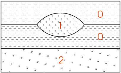
The easiest way to describe geologic hierarchy is with an example. Consider the example below of a clay lens in sand with gravel below. Some borings will see only sand above the gravel, while others will reveal an upper sand, clay, and lower sand.

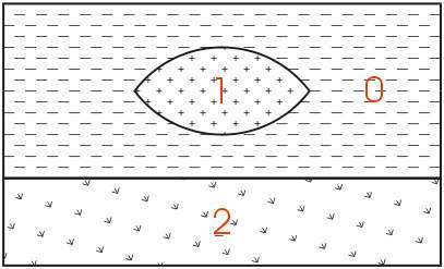
The geologic hierarchy for this site will be upper sand, clay, lower sand, and gravel. This requires that the borings with only sand (above the gravel) be described as upper sand, clay, and lower sand, with the clay described as being zero thickness. For this simple example, determining the hierarchy is straightforward. For some sites (as will be discussed later) it is very difficult or even impossible.

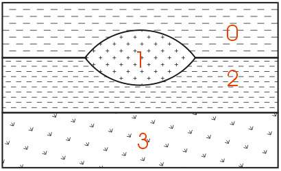
For those sites that can be described using the above method, it remains the best approach for building a 3D geologic model. Each layer has smooth boundaries and the layers (by nature of hierarchy) can be exploded apart to reveal the individual layer surface features. In the above example, the numbers represent the layer numbers for this site (even though layers 0 and 2 are both sand). Two examples of much more complex sites that are best described by this original approach are shown below.

Geologic Example: Sedimentary Layers and Lenses

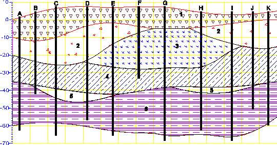
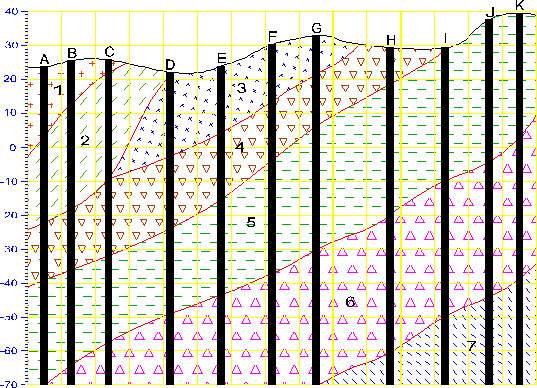
Geology Example & Figure: Outcrop of Dipping Strata

EVS is not limited to sedimentary layers or lenses. The figure below shows a cross-section through an outcrop of dipping geologic strata. EVS can easily model the layers truncating on the top ground surface.

However, many sites have geologic structures (plutons, karst geology, sand channels, etc.) that do not lend themselves to description within the context of hierarchical layers. For these sites, Geologic Indicator Kriging (GIK) offers the ability to build extremely complex models with a minimum of effort (and virtually no interpretation) on the part of the geologist. GIK can also be a useful check of geologic hierarchies developed for sites that do lend themselves to a model based upon hierarchical layers.

GIK uses raw, uninterpreted 3D borings logs as the input file. The .pgf (pre-geology file) format is used to represent these logs. PGF files contain descriptions of each boring with x,y, & z coordinates for ground surface and the bottom of each observed geologic unit. Consecutive integer values (e.g. 0 through n-1, for n total observed units in the site) are used to describe each material observed in the entire site.

NOTE: It is important to start your material ID numbering at zero (0) instead of 1.

Usually, materials are numbered based upon a logical classification (such as porosity or particle size), however the numbering can be arbitrary as long as the numbers are consecutive (don’t leave numbers out of the sequence). For the example given above, we could number the materials as shown in the figure below (even though it is not a numbering sequence based on porosity or particle size).

For a .pgf file, borings that do not see the clay (material 2 in the figure) would not need to consider the sand as being divided into upper and lower. Rather, every boring is merely a simple ASCII representation of the raw borings logs. The only interpretation involves classification of the observed soil types in each boring and assigning an associated numbering scheme.

mask horizons

mask horizons receives geologic input into its left input port and an optional input masking surface into its right port.

Module Input Ports

• Input Field [Field] Accepts a data field.
• Input Area [Field] Accepts a field defining a surface of the area for masking

Module Output Ports

• Output Field [Field] Outputs the processed field.

NOTE: The mask is normally applied to the first surface only. If this surface is removed, the mask is lost. However the “Allow Subsetting” toggle will apply the mask to all horizons, but it will slow down processing and use more memory.

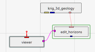
edit_horizons is an interactive module which allows you to probe points to be selectively added to the creation of each and every stratigraphic horizon. This provides the ability to manual edit horizon surfaces prior to the creation of geologic models.

The method of connecting edit_horizons is unique among our modules. It uses the pink output port from gridding and horizons as its primary input, and it also requires the purple side port from viewer since it requires interactive probing. Its blue output port then becomes equivalent to the blue output of gridding and horizons, but with edited surfaces.

Regardless of the estimation method used originally, edit_horizons uses Natural Neighbor to perform its near-real-time modifications. For this reason, there is a Use Gradients toggle at the top of the user interface, which is identical in function to the one in gridding and horizons.

The other important parameter at the top of the user interface is the Horizon Point Radius. The default (linked) value for this parameter is computed for you as 2% of the X-Y diagonal extents of your input geology. If any of the original data points for the selected horizon being edited fall within the Horizon Point Radius, then we don’t use your probed point based on the assumption that the original data is more defensible and should take precedence.

Next there is the Probe Action, which has 3 options:

1. None (default state when the module is instanced)
2. Reset Position (allows you to move points)
3. Add Point (allows you to add new surface control points for the selected horizon)

The Horizons list shows all of your geologic horizons. Here, you select the horizon surface you wish to modify. The points that you add only affect the selected horizon. When you change the selected horizon, you can add new points for that surface. You are able to add as many points as you need for any or all of the horizons.

The Horizon Point List is the list of points that you have added by probing in your model. You can only probe on actual objects. These objects can be surfaces from horizons, slices, tubes, or whatever objects you’ve added to your viewer. Slices are very useful since you can move them where you need them so you can probe points at specific coordinates. You are also able to manually change the X, Y, and/or Z coordinates or any point as needed. For each point, a Note: box is provided so you can keep a record of your actions and reasons.

horizon_ranking

The horizon_ranking module is used to give the user control over individual surface priorities and rankings. This allows the user to fine tune their hierarchy in ways much more complex than a simple top-down or bottom-up approach.

Module Input Ports

horizon_ranking has one input port which receives geologic input from modules like gridding and horizons

Module Output Ports

horizon_ranking has one output port which outputs the geologic input with re-prioritized hierarchy

Module Input Ports

• Input Field [Field] Accepts a data field from 3d estimation or other similar modules.

Module Output Ports

• Output Field [Field] Outputs the subsetted field as edges
• Geologic legend Information [Geology legend] Outputs the geologic material information

material_mapping

This module can re-assign data corresponding to:

• Geologic Layer
• Material ID
• Indicator
• Adaptive Indicator

for the purpose of grouping. This provides great flexibility for exploding models or coloring.

Groups are processed from Top to Bottom. You can have overlapping groups or groups whose range falls inside a previous group. In that event, the lower groups override the values mapped in a higher group.

For example, if you have ten material ids (0 through 9) and you want to have them all be 0 except for 5 & 6 which should be 1, this can be accomplished with two groups:

1. From 0 to 9 Map to 0
2. From 5 to 6 Map to 1

Please note that in the animator, you can animate these values. Each group has From, To and Map To values that are numbered zero through eleven (e.g. From0, MapTo5)

Module Input Ports

• Input Field [Field] Accepts a data field.

Module Output Ports

• Output Field [Field] Outputs the processed field.

combine horizons

The combine horizons module is used to merge up to six geologic horizons (surfaces) to create a field representing multiple geologic layers.

The mesh (x-y coordinates) from the first input field, will be the mesh in the output. The input fields should have the same scale and origin, and number of nodes in order for the output data to have any meaning.

It also has a Run toggle (to prevent downstream modules from firing during input setting changes).

combine horizons provides an important ability to merge sets of surfaces or add additional surfaces to geologic models. It is important to understand the consequences of doing so and the steps that must be taken. The Brown-Grey-Light Brown-Beige port contains the material_ID numbers and names and it is important that the content of this port reflect the current set of surfaces/layers reflected in the geology. When Material_ID or Geo_Layer is presented in a legend, this port is necessary to automatically provide the layer names. When combine horizons is used to construct modified geologic horizons, its Geologic legend Information port MUST be used vs. the same port in gridding and horizons

Module Input Ports

• Input Geologic Field [Field] Accepts a field with data whose grid will be exported.
• Input Field 1 [Field] Accepts a data field.
• Input Field 2 [Field] Accepts a data field.
• Input Field 3 [Field] Accepts a data field.
• Input Field 4 [Field] Accepts a data field.
• Input Field 5 [Field] Accepts a data field.

Module Output Ports

• Geologic legend Information [Geology legend] Supplies the geologic material information for the legend module.
• Output Geologic Field [Field] Outputs the field with selected data
• Output Object [Renderable]: Outputs to the viewer.

subset horizons

The subset horizons module allows you to subset the output of gridding and horizons so that downstream modules (3d estimation, horizons to 3d, Geologic Surface) act on only a portion of the layers kriged.

subset horizons is used to select a subset of the layers (and corresponding surfaces) export from gridding and horizons. This is useful if you want (need) to krige parameter data in each geologic layer separately.

This is not normally needed with contaminant data, but when you are kriging data such as porosity that is inherently discontinuous across layer boundaries, it is essential that each layer be kriged with data collected ONLY within that layer.

subset horizons eliminates the need for multiple gridding and horizons modules reading data files that are subsets of a master geology. Inserting subset horizons between gridding and horizons and 3d estimation allows you to select one or more layers from the geology.

This functionality is very useful when you want to krige groundwater and soil data using a single master geology file that represents both the saturated and unsaturated zones.

Module Input Ports

• Input Geologic Field [Field] Accepts a data field from gridding and horizons to krige data into geologic layers.

Module Output Ports

• Geologic legend Information [Geology legend] Supplies the geologic material information for the legend module.
• Output Geologic Field [Field] Can be connected to the 3d estimation, 3D_Geology Map, and surface from horizons(s) modules.

collapse horizons

The collapse horizons module allows you to subset the output of gridding and horizons so that downstream modules (3d estimation, horizons to 3d, Geologic Surface) act on only a single merged layer.

collapse horizons is used to merge all layers (and corresponding surfaces) export from gridding and horizons into a single layer (topmost and bottommost surfaces).

collapse horizons eliminates the need for multiple gridding and horizons modules reading data files that are single layer subset of a master geology. Inserting collapse horizons between gridding and horizons and 3d estimation kriges all data into a single geologic layer. When used with subset horizons it allows for creating a single layer that represents a only a portion (subset) of the master geology file.

Module Input Ports

• Input Geologic Field [Field] Accepts a data field from gridding and horizons to krige data into geologic layers.

Module Output Ports

• Geologic legend Information [Geology legend] Supplies the geologic material information for the legend module.
• Output Geologic Field [Field] Can be connected to the 3d estimation, 3D_Geology Map, and surface from horizons(s) modules.

displace_block

displace_block receives any 3D field into its input port and outputs the same field translated in z according to a selected nodal data component of an input surface allowing for non-uniform fault block translation.

This module allows for the creation of tear faults and other complex geologic structures. Used in conjunction with distance to surface it makes it possible to easily model extremely complex deformations.

Module Input Ports

• Input Field [Field] Accepts a volumetric field
• Input Surface [Field] Accepts a 2D surface grid with elevation nodal data. This type of grid is created by gridding and horizons and import raster as horizon.

Module Output Ports

• Output Field [Field] Outputs the displaced field
• Output Object [Renderable]: Outputs to the viewer.