3d estimation

3d estimation performs parameter estimation using kriging and other methods to map 3D analytical data onto volumetric grids defined by the limits of the data set, or by the convex hull, rectilinear, or finite-difference grid extents of a geologic system modeled by gridding and horizons. 3d estimation provides several convenient options for pre- and post-processing the input parameter values, and allows the user to consider anisotropy in the medium containing the property.

3d estimation also has the ability to create uniform fields, and the ability to choose which data components you want to include in the output. There are a couple significant requirements for uniform fields. First, there cannot be geologic input (otherwise the cells could not be rectangular blocks). Second, Adaptive_Gridding must be turned off (otherwise the connectivity is not implicit).

Module Input Ports

• Filename [String / minor] Allows the sharing of file names between similar modules.
• Input Geologic Field [Field] Accepts a data field from gridding and horizons to krige data into geologic layers.
• Input External Grid [Field / minor] Allows the user to import a previously created grid. All data will be kriged to this grid.
• Input External Data [Field / minor] Allows the user to import a field contain data. This data will be kriged to the grid instead of using file data.

Module Output Ports

• Filename [String / minor] Allows the sharing of file names between similar modules.
• Output Field [Field] Outputs a 3D data field which can be input to any of the Subsetting and Processing modules.
• Status Information [String / minor] Outputs a string containing module parameters. This is useful for connection to write evs field to document the settings used to create a grid.
• Uncertainty Sphere [Renderable / minor] Outputs a sphere to the viewer. This sphere represents the location of maximum uncertainty.

Properties and Parameters

The Properties window is arranged in the following groups of parameters:

• Grid Settings: control the grid type, position and resolution
• Data Processing: controls clipping, processing (Log) and clamping of input data and kriged outputs.
• Time Settings: controls how the module deals with time domain data
• Krig Settings: control the estimation methods
• Data To Export: specify which data is included in the output
• Display Settings: applies to maximum uncertainty sphere
• Drill Guide: parameters association with DrillGuide computations for analytically guided site assessment

Variogram Options:

There are three variogram options:

1. Spherical: Our default and recommended choice for most applications
2. Exponential: Generally gives similar results to Spherical and may be superior for some datasets
3. Gaussian: Notoriously unstable, but can “smooth” your data with an appropriate nugget.

I specifically want to discuss the pros and cons of Gaussian. Without a nugget term, Gaussian is generally unusable. When using Autofit, our expert system will apply a modest nugget (~1% of sill) to maintain stability. If you’re committed to experimenting with Gaussian, it is recommended that you experiment with the nugget term after EVS computes the Range and Sill. Below are some things to look for:

• If you find that Gaussian kriging is overshooting the plume in various directions, your nugget is likely too small.
• However, if the plume looks overly smooth and is too far from honoring your data, your nugget is likely too big.

The “Power Factor” is only used for exponential or gaussian variograms. The default value of 3 is the most common value used for exponential in most software. For gaussian, 2 is most common, though anything from 0.1->3 is typically acceptable. This is effectively the “a” term described here: https://en.wikipedia.org/wiki/Variogram#Variogram_models

Advanced Variography Options:

It is far beyond the scope of our Help documentation to include an advanced Geostatistics course. The terminology and variogram plotting style that we use is industry standard and we do so because we will not provide detailed technical support nor complete documentation on these features, which would effectively require a geostatistics textbook, in our help.

However, there is an Advanced Training Video on how to take advantage of the complex, directional anisotropic variography capabilities in 3d estimation (which applies equally well to lithologic modeling). This class is focused on the mechanics of how to employ and refine the variogram anisotropy with respect to your data and the physics of your project such as contaminated sediments in a river bottom. The variogram is displayed as an ellipsoid which can be distorted to represent the Primary and Secondary anisotropies and rotated to represent the Heading, Dip and Roll. Overall scale and translation are also provided as additional visual aids to compare the variogram to the data, though these do not affect the actual variogram.

We are not hiding this capability from you as the Anisotropic Variography Study folder of Earth Volumetric Studio Projects contains a number of sample applications which demonstrate exactly what is described above. However, we assure you that understanding how to apply this to your own projects will be quite daunting and really does require a number of prerequisites:

• A thorough explanation of these complex applications
• An understanding of all of the variogram parameters and their impact on the estimation process on both theoretical datasets as well as real-world datasets.

This 3 hour course addresses these issues in detail.

2d estimation

2d estimation performs parameter estimation using kriging and other methods to map 2D analytical data onto surface grids defined by the limits of the data set as rectilinear or convex hull extents of the input data.

Its Adaptive Griddingfurther subdivides individual elements to place a “kriged” node at the location of each input data sample. This guarantees that the output will accurately reflect the input at all measured locations (i.e. the maximum in the output will be the maximum of the input).

The DrillGuide functionality produces a new input data file with a synthetic boring at the location of maximum uncertainty calculated from the previous kriging estimates, which can then be rerun to find the next area of highest uncertainty. The naming of the “DrillGuide^©” file which is created when 2d estimation is run with all types of analyte (e.g. chemistry) files ends in apdv1, apdv2, apdv3, etc. the output file name will be .apdv2, apdv3, apdv4…. There are no limits to the number of cycles that may be run.

The use of 2d estimation to perform analytically guided site assessment is covered in detail in Workbook 2: DrillGuide^© Analytically Guided Site Assessment.

This process can be continued as many times as desired to define the number and placement of additional borings that are needed to reduce the maximum uncertainty in the modeled domain to a user specified level. The features of 2d estimation make it particularly useful for optimizing the benefits obtained from environmental sampling or ore drilling programs. 2d estimation also provides some special data processing options that are unique to it, which allow it to extract 2-dimensional data sets from input data files that contain three-dimensional data. This functionality allows it to use the same .apdv files as all of the other EVS input and kriging modules, and allows detailed analyses of property characteristics along 2-dimensional planes through the data set. 2d estimation also provides the user with options to magnify or distort the resulting grid by the kriged value of the property at each grid node. 2d estimation also allows the user to automatically clamp the data distribution to a specified level along a boundary that can be offset from the convex hull of the data domain by a user defined amount.

Module Input Ports

• Input External Grid [Field / minor] Allows the user to import a previously created grid. All data will be kriged to this grid.
• Input External Data [Field / minor] Allows the user to import a field contain data. This data will be kriged to the grid instead of using file data.
• Filename [String / minor] Allows the sharing of file names between similar modules.

Module Output Ports

• Output Field [Field] Outputs a 3D data field which can be input to any of the Subsetting and Processing modules which have the same color port
• Filename [String / minor] Allows the sharing of file names between similar modules.
• Status Information [String / minor] Outputs a string containing module parameters. This is useful for connection to write evs field to document the settings used to create a grid.
• Surface [Renderable] Outputs the kriged surface to the viewer

Properties and Parameters

The Properties window is arranged in the following groups of parameters:

• Grid Settings: control the grid type, position and resolution
• Data Processing: controls clipping, processing (Log) and clamping of input data and kriged outputs.
• Time Settings: controls how the module deals with time domain data
• Krig Settings: control the estimation methods
• Data To Export: specify which data is included in the output
• Display Settings: applies to maximum uncertainty sphere
• Drill Guide: parameters association with DrillGuide computations for analytically guided site assessment

Variogram Options:

There are three variogram options:

1. Spherical: Our default and recommended choice for most applications
2. Exponential: Generally gives similar results to Spherical and may be superior for some datasets
3. Gaussian: Notoriously unstable, but can “smooth” your data with an appropriate nugget.

I specifically want to discuss the pros and cons of Gaussian. Without a nugget term, Gaussian is generally unusable. When using Autofit, our expert system will apply a modest nugget (~1% of sill) to maintain stability. If you’re committed to experimenting with Gaussian, it is recommended that you experiment with the nugget term after EVS computes the Range and Sill. Below are some things to look for:

• If you find that Gaussian kriging is overshooting the plume in various directions, your nugget is likely too small.
• However, if the plume looks overly smooth and is too far from honoring your data, your nugget is likely too big.

gridding and horizons

The gridding and horizons module uses data files containing geologic horizons or surfaces (usually .geo, .gmf and other ctech formats containing surfaces) to model the surfaces bounding geologic layers that will provide the framework for three-dimensional geologic modeling and parameter estimation. Conversion of scattered points to surfaces uses kriging (default) or spline (previously in the spline_geology module), IDW or nearest neighbor algorithms.

gridding and horizons creates a 2D grid containing one or more elevations at each node. Each elevation represents a geologic surface at that point in space. The output of gridding and horizons is a data field that can be sent to several modules (e.g. 3d estimation, horizons to 3d, horizons_to_3d_structured, surfaces from horizons, etc.)

Those modules which create volumetric models convert the quadrilateral elements into layers of hexahedral (8-node brick) elements. The output of gridding and horizons can also be sent to the surface from horizons(s) module(s) which allow visualization of the individual layers of quadrilateral elements (the surfaces) that comprise the surfaces.

gridding and horizons has the capability to produce layer surfaces within the convex hull of the data domain, within a rectilinear domain with equally spaced nodes, or within a rectilinear domain with specified cell sizes such as a finite-difference model grid. The finite-difference gridding capabilities allows the user to visually design a grid with variable spacing, and then krige the geologic layer elevations directly to the finite difference grid nodes. gridding and horizons also provides geologic surface definitions to the post_samples module to allow exploding of boreholes and samples by geologic layer.

Note: gridding and horizons has the ability to read .apdv, .aidv and .pgf file to create a single geologic layer model. This was not done as a preferred alternative to creating/representing your valid site geology. However, most sites have some ground surface topography variation. If 3d estimation is used without geology input, the resulting output will have flat top and bottom surfaces. The flat top surface may be below or above the actual ground surface at various locations. This can result in plume volumes that are inaccurate.

When a .apdv or .pgf is read by gridding and horizons the files are interpreted as geology as follows:

1. If Top of boring elevations are provided in the file, these values are used to create the ground surface.

2. If Top of boring elevations are not provide in the file, the elevations of the highest sample in each boring are used to create the ground surface.

3. The bottom surface is created as a flat surface slightly below the lowest sample in the file. The elevation of the surface is computed by taking the lowest sample and subtracting 5% of the total z-extent of the samples.

When reading these files, you will get a single layer which goes to either the Top column (if it exists) otherwise, the top sample in each boring, and 5% below the lowest sample in the file (flat bottom). This allows you to create a convex hull around data without having geology info. It also provide a topographic top surfaces if your analyte (e.g. chemistry) or PGF file has Tops (grounds surface elevations). Also nice for doing indicator kriging (since a single, well-defined pgf can give you an entire indicator model now). Be aware that if Top is specified, but all values are exactly 0.0, the top sample elevation for each boring will be used.

Module Input Ports

• Filename [String / minor] Receives the filename from other modules.

Module Output Ports

• Geologic legend Information [Geology legend] Supplies the geologic material information for the legend module.
• Output Geologic Field [Field] Can be connected to the 3d estimation, 3D_Geology Map, and surface from horizons(s) modules.
• Filename [String / minor] Outputs a string containing the file name and path. This can be connected to other modules to share files.
• Status Information [String / minor] Outputs a string containing module parameters. This is useful for connection to write evs field to document the settings used to create a grid.
• Geology Export Output [Vistas Data / minor] Provides input to the export horizons to vistas and other modules which create raster output.
• Grid [Renderable / minor] Outputs the geometry of 2D grid.

Properties and Parameters

The Properties window is arranged in the following groups of parameters:

• Grid Settings: control the grid type, position and resolution
• Krig Settings: control the estimation methods
• Computational Settings: define computational surfaces included in the output. This allows a single surface file to define a layer specified by elevation or depth.

analytical realization

The analytical realization module is one of three similar modules (the other two are lithologic realization and stratigraphic_realization), which allows you to very quickly generate statistical realizations of your 2D and 3D kriged models based upon C Tech’s Proprietary Extended Gaussian Geostatistical Simulation (GGS) technology, which we refer to as Fast Geostatistical Realizations^^®^ or FGR^^®^. Our extensions to GGS allow you to:

• Create realizations very rapidly
• Exercise greater control over the frequency and magnitude of noise typical in GGS.
• Control deviation magnitudes from the nominal kriged prediction based on a Min Max Confidence Equivalent.
  • Deviations are the absolute value of the changes to the analytical prediction (in user units)
• Apply Simple or Advanced Anisotropy control over 2D or 3D wavelengths

C Tech’s FGR^^®^ creates more plausible cases (realizations) which allow the Nominal concentrations to deviate from the peak of the bell curve (equal probability of being an under-prediction as an over-prediction) by the same user defined Confidence. However, FGR allows the deviations to be both positive (max) and negative (min), and to fluctuate in a more realistic randomized manner.

Module Input Ports

• Realization [Special Field] Accepts outputs from 3d estimation and krig_2d to allow for EGGS models to be created

Module Output Ports

• Output Field [Field] Outputs the subsetting level
• Deviations Field [Field] Outputs the deviations from the nominal kriged model

Important Parameters

There are several parameters which affect the realizations. A brief description of each follows:

• Randomness Generator Type
  • There are four types, each of which create a different 2D/3D random distribution
• Anisotropy Mode
  • Two options here are Simple or Advanced. These are equivalent to the variogram settings in 3d estimation or krig_2d
• Seed
  • The “Seed” is used in the random number generator, and makes it reproducible.
  • Unique seeds create unique realizations
• Wavelength
  • The 2D or 3D random distribution is governed by a mean wavelength that determines the apparent frequency of deviations from the nominal kriged result.
  • Wavelength is in your project coordinates (e.g. meters or feet)
  • Longer wavelengths create smoother realizations
  • Shorter wavelengths create more “noisy” variations in the realizations
  • Very short wavelengths will give results more similar to GGS (aka Sequential Gaussian Simulations)
• Min Max Confidence Equivalent
  • This parameter determines the magnitude of the deviations.
  • Values close to 50% result in outputs that deviate very little from the nominal kriged result.
    • (we do not allow values below 51% for algorithm stability reasons)
  • Values at or approaching 99.99% will result in the greatest (4 sigma) variations (more similar to GGS)

stratigraphic realization

The stratigraphic realization module is one of three similar modules (the other two are analytical_realization and lithologic realization), which allows you to very quickly generate statistical realizations of your stratigraphic horizons based uponC Tech’s Proprietary Extended Gaussian Geostatistical Simulation (GGS), which we refer to as Fast Geostatistical Realizations^^®^ or FGR^^®^. Our extensions to GGS allow you to:

• Create realizations rapidly
• Exercise greater control over the frequency and magnitude of noise typical in GGS.
• Control deviation magnitudes from the nominal kriged prediction based on a Min Max Confidence Equivalent.
  • Deviations are the absolute value of the changes to surface elevations for each stratigraphic horizon.
• Apply Simple or Advanced Anisotropy control over 2D wavelengths
• For stratigraphic realizations only: we support Natural Neighbor as well as kriging for the input model.

Module Input Ports

• Realization [Special Field] Accepts outputs from gridding and horizons to allow for FGR^^®^ models to be created

Module Output Ports

• Output Field [Field] Outputs the subsetting level
• Deviations Field [Field] Outputs the deviations from the nominal kriged model

Important Parameters

There are several parameters which affect the realizations. A brief description of each follows:

• Randomness Generator Type
  • There are four types, each of which create a different 2D/3D random distribution
• Anisotropy Mode
  • Two options here are Simple or Advanced. These are equivalent to the variogram settings in gridding and horizons
• Seed
  • The “Seed” is used in the random number generator, and makes it reproducible.
  • Unique seeds create unique realizations
• Wavelength
  • The 2D or 3D random distribution is governed by a mean wavelength that determines the apparent frequency of deviations from the nominal kriged (or Natural Neighbor) result.
  • Wavelength is in your project coordinates (e.g. meters or feet)
  • Longer wavelengths create smoother realizations
  • Shorter wavelengths create more “noisy” variations in the realizations
  • Very short wavelengths will give results more similar to GGS (aka Sequential Gaussian Simulations)
• Min Max Confidence Equivalent
  • This parameter determines the magnitude of the deviations.
  • Values close to 50% result in outputs that deviate very little from the nominal kriged (or Natural Neighbor) result.
    • (we do not allow values below 51% for algorithm stability reasons)
  • Values at or approaching 99.99% will result in the greatest (4 sigma) variations (more similar to GGS)

lithologic realization

The lithologic realization module is one of three similar modules (the other two are analytical_realization and stratigraphic_realization), which allows you to very quickly generate statistical realizations of your 2D and 3D lithologic models based upon C Tech’s Proprietary Extended Gaussian Geostatistical Simulation (GGS), which we refer to as Fast Geostatistical Realizations^^®^ or FGR^^®^. Our extensions to GGS allow you to:

• Create realizations rapidly:
  • Though indicator_realizations are the slowest of the three because:
  • The material probabilities must be additionally processed to assign materials
  • When Smooth option is on, this process often takes nearly as long as the original kriging
• Exercise greater control over the frequency and magnitude of visual noise typical of GGS.
• Control deviation magnitudes from the nominal kriged probability prediction based on a Min Max Confidence Equivalent.
  • Deviations are the absolute value of the changes to each material’s probability
• Apply Simple or Advanced Anisotropy control over 2D or 3D wavelengths

Module Input Ports

• Realization [Special Field] Accepts outputs from 3d estimation and krig_2d to allow for EGGS models to be created

Module Output Ports

• Output Field [Field] Outputs the subsetting level
• Deviations Field [Field] Outputs the deviations from the nominal kriged probabilities

Important Parameters

There are several parameters which affect the realizations. A brief description of each follows:

• Randomness Generator Type
  • There are four types, each of which create a different 2D/3D random distribution
• Anisotropy Mode
  • Two options here are Simple or Advanced. These are equivalent to the variogram settings in lithologic modeling
• Seed
  • The “Seed” is used in the random number generator, and makes it reproducible.
  • Unique seeds create unique realizations
• Wavelength
  • The 2D or 3D random distribution is governed by a mean wavelength that determines the apparent frequency of deviations from the nominal kriged probabilities results.
  • Wavelength is in your project coordinates (e.g. meters or feet)
  • Longer wavelengths create smoother realizations
  • Shorter wavelengths create more “noisy” variations in the realizations
  • Very short wavelengths will give results more similar to GGS (aka Sequential Gaussian Simulations)
• Min Max Confidence Equivalent
  • This parameter determines the magnitude of the deviations.
  • Values close to 50% result in outputs that deviate very little from the nominal kriged probabilities results.
    • (we do not allow values below 51% for algorithm stability reasons)
  • Values at or approaching 99.99% will result in the greatest (4 sigma) variations (more similar to GGS)

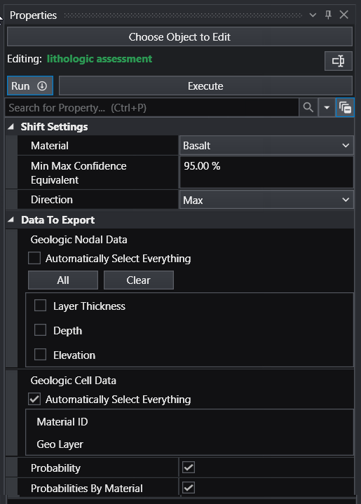
Lithologic assessment provides a way to determine the quality of a lithologic model on an individual material basis. The concept and procedure to do this is:

• Select the material to be assessed (Basalt shown below)

• Choose a Min Max Confidence Equivalent value (95% shown below)

  • A 50% confidence will result in the Min or Max being equal to the nominal model
  • High confidence values (90+%) will show greater difference from nominal

• Select the Direction (Max or Min)

• Choose the data to be exported

Module Input Ports

• Realization [Special Field] Accepts output from lithologic modeling

Module Output Ports

• Output Field [Field] Outputs the subsetting level
• Deviations Field [Field] Outputs the deviations from the nominal kriged probabilities

external_kriging

The external_kriging module allows users to perform estimation using grids created in EVS (with our without layers or lithology) in GeoEAS which supports very advanced variography and kriging techniques. Grids and data are kriged externally from EVS and the results can then be read into EVS and treated as if they were kriged in EVS.

This an advanced module which should be used only by persons with experience with GeoEAS and geostatistics. C Tech does not provide tech support for the use of GeoEAS.

Module Input Ports

• Z Scale [Number] Accepts Z Scale (vertical exaggeration) from other modules
• Input Data [Field] Allows the user to import a field contain data. This data will be kriged to the grid instead of using file data.
• Input Grid [Field] Allows the user to import a previously created grid. All data will be kriged to this grid.

Module Output Ports

• Output [Field] Outputs a 3D data field which can be input to any of the Subsetting and Processing modules.

Properties and Parameters

The Properties window is arranged in the following groups of parameters:

• Properties: defines Z Scale and grid translation(s)
• Export Data: controls the file names and data processing for creation of GeoEAS inputs.
• Export Grid: Exports the grid and data to GeoEAS formats. A grid and data must be connected to the import ports
• Import Data: Imports the grid and data to GeoEAS formats. A grid and data must be connected to the import ports