scat_to_unif The scat_to_unif module is used to convert scattered sample data into a three-dimensional uniform field. Also, scat_to_unif can be used to take an existing grid (for example a UCD file) and convert it to a uniform field. scat_to_unif converts a field of non-uniformly spaced points into a uniform field which can be used with many of EVS’s filter and mapper modules. “Scattered sample data " means that there are disconnected nodes in space. An example would be geology or analyte (e.g. chemistry) data where the coordinates are the x, y, and elevation of a measured parameter. The data is “scattered” because there isn’t data for every x/y/elevation of interest.
merge_fences The merge_fences module is used to merge the output from multiple krig_fence modules into one data set (i.e., to merge cross sections into a fence diagram). This is useful for performing uniform data manipulation procedures on fence data from several krig_fence outputs. For example, if several krig_fence modules are used, they should all pass through a merge_fences module before being passed to explode and scale. Therefore, all fences will be exploded and scaled the same amount and only one dialog box is needed to control all fences. merge_fences should always be used when more than one krig_fence module is used.
project_field General Module Function The project_field module is used to project the coordinates in any field, from one coordinate system to another. Module Control Panel The control panel for project_field is shown in the figure above. Each coordinate system is divided into either Geographic or Projected coordinate systems. The coordinate system types are navigated by selecting the appropriate system type in the far left window. When a general coordinate system has been selected a specific coordinate system can be selected from the center window. If there are any details regarding the selected specific coordinate system, they will appear in the text window on the right. A specific coordinate system must be selected both to project from and to project to as in the picture below.
geologic_surfmap This module is deprecated and replaced by project onto surface. geologic_surfmap provides a mechanism to drape lines onto Geologic surfaces. It compares to project onto surface, but lines are not subsetted to match the size of the cells of the surface on which the lines are draped. In other words, only the endpoints of each line segment are draped.
time_field The time_field module allows you to extract a field (grid with data) from a set of time-based fields. The time for the extracted field can be any time between the start and end of the set of fields. It will interpolate between adjacent known times.
video_safe_area The video_safe_area module is used when creating an animation for DVD or Video. It displays the areas that are usable for both text and animation purposes for several standard video formats. This allows you to properly setup your animation in order to get the best possible output on multiple television sets.
advector The advector module combines streamlines capability and a tool for sequential positioning of glyphs along the streamlines trajectory to simulate advection of weightless particles through a vector field (for example, a fluid flow simulation such as modflow). The result is an animation of particle motion, with the particles represented as any EVS geometry (such as a jet or a sphere). The glyphs can scale, deflect or deform according to the velocity vector it passes. At least one of the nodal data components input to advector must be a vector. The direction of travel of streamlines can be specified to be forwards (toward high vector magnitudes) or backwards (toward low vector magnitudes) with respect to the vector field. The input glyphs travel along streamlines (not necessarily visible in the viewer) which are produced by integrating a velocity field using the Runge-Kutte method of specified order with adaptive time steps.
modpath_advector The modpath_advector module combines MODPATH capability and a tool for sequential positioning of glyphs along the MODPATH lines trajectory to simulate advection of weightless particles through a vector field. The result is an animation of particle motion, with the particles represented as any EVS geometry (such as a jet or a sphere). The glyphs can scale, deflect or deform according to the velocity vector it passes. The direction of travel of streamlines can be specified to be forwards (toward high vector magnitudes) or backwards (toward low vector magnitudes) with respect to the vector field. The input glyphs travel along streamlines (not necessarily visible in the viewer) which are produced by integrating a velocity field using the Runge-Kutte method of specified order with adaptive time steps.
read symbols The read symbols module creates symbolic representations of different borehole identifiers based on a set of user defined parameters. The symbols are displayed at the top of the each borehole based on its x,y & z coordinates. A sample file with 48 predefined symbols is included, but it can be customized to produce special symbols.
create_spheroid This module is deprecated and replaced by place_glyph The create_spheroid module produces a 2D circular disc or 3D spheroidal or ellipsoidal grid that can be used for any purpose, however the primary application is as starting points for 3d streamlines or advector. Module Input Ports Input Field [Field] Accepts a field to extract its extent Module Output Ports
advect_surface The advect_surface module combines surface streamlines capability and a tool for sequential positioning of glyphs along the streamlines trajectory to simulate advection of particles down a surface. The result is an animation of particle motion, with the particles represented as any EVS geometry (such as a jet or a sphere). The glyphs can scale, deflect or deform according to the velocity vector. The direction of travel of streamlines can be specified to be downhill or uphill (for the slope case). The input glyphs travel along streamlines (not necessarily visible in the viewer) which are produced by integrating a velocity field using the Runge-Kutte method of specified order with adaptive time steps.
fence_geology The fence_geology module uses data in specially formatted .geo files to model the surfaces of geologic layers in vertical planes, or cross sections. Fence Geology essentially creates layers of quadrilateral (4 node) elements (in a vertical plane) in which each node (and element) is assigned to an individual geologic layer. The output of fence_geology is a data field, consisting of a 2D line with each layers elevation as nodal data elements, that can be sent to the krig_fence and horizons to 3d modules where the quadrilateral elements are connected to the element nodes in adjacent geologic surfaces to create layers along the fence.
file_output The file_output module creates a formatted string based upon the values passed to it. This string is then written to the selected ascii text file. Certain modules such as 3d estimation, krig_2d, and krig_fence output a formatted string for just this purpose.
adaptive_indicator_krig adaptive_indicator_krig is an alternative geologic modeling concept that uses geostatistics to assign each cell’s lithologic material as defined in a pregeology (.pgf) file, to cells in a 3D volumetric grid. There are two methods of lithology assignment: Nearest Neighbor is a quick method that merely finds the nearest lithology sample interval among all of your data and assigns that material. It is very fast, but generally should not be used for your final work. Kriging provides the rigorous probabilistic approach to geologic indicator kriging. The probability for each material is computed for each cell center of your grid. The material with the highest probability is assigned to the cell. All of the individual material probabilities are provided as additional cell data components. This will allow you to identify regions where the material assignment is somewhat ambiguous. Needless to say, this approach is much slower (especially with many materials), but often yields superior results and interesting insights. adaptive_indicator_krig is an extension of the technology in lithologic modeling for several reasons:
krig_fence krig_fence models parameter distributions within domains defined by the boundaries of the input data in 3D Fence sections which can “snake” around in the x-y plane and are parallel to the z-axis. krig_fence can also receive the geologic system modeled by Fence Geology. It creates a quadrilateral finite-element grid with kriged nodal values of any scalar property and its kriged confidence level, and outputs a geometry whose elements can be rendered to view the color scaled parameter distribution on the element surfaces. krig_fence provides several convenient options for pre- and post-processing the input parameter values, and allows the user to consider anisotropy in the medium containing the property.
fence_geology_map The fence_geology_map module creates 3-dimensional fence diagram from the 1-dimensional line contours which follow your geology produced by fence_geology, to allow visualizations of the geologic layering of a system. It accomplishes this by creating a user specified distribution of nodes in the Z dimension between the top and bottom lines defining each geologic layer. The number of nodes specified for the Z Resolution may be distributed (proportionately) over the geologic layers in a manner that is approximately proportional to the fractional thickness of each layer relative to the total thickness of the geologic domain. In this case, at least three layers of nodes (2 layers of elements) will be placed in each geologic layer.
application_notes The application_notes has been deprecated and replaced by the Annotation’s “Notes”
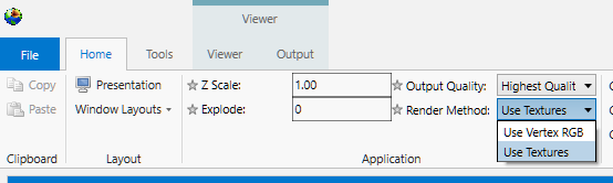
texture_colors This is a deprecated module texture_colors functionality has been incorporated into all modules. On the Home tab, you have the Render Method selector where you can choose to use Vertex RGB coloring or Textures.
texture_wave The texture_wave module utilizes transparency and texture mapping similar to texture_colors and illuminated_lines technology to create an animated effect. However, unlike illuminated_lines, this module works with both OpenGL and Software Rendering. texture_wave has a single input port that accepts the grid with nodal data that you want to color with this technique. This would normally be tubes or streamribbons.
illuminated_lines Display of Illuminated Lines using texture mapped illumination model on polylines with line halo and animation effects. Prerequisites This module requires OpenGL rendering to be selected. This module utilizes special OpenGL calls to implement the illuminated line technique. If this module is used with another renderer, such as the software renderer or the output_images module (not set to Automatic), lines will be drawn in the default mode with illuminated line features disabled.
Subsections of Deprecated
scat_to_unif
The scat_to_unif module is used to convert scattered sample data into a three-dimensional uniform field. Also, scat_to_unif can be used to take an existing grid (for example a UCD file) and convert it to a uniform field. scat_to_unif converts a field of non-uniformly spaced points into a uniform field which can be used with many of EVS’s filter and mapper modules. “Scattered sample data " means that there are disconnected nodes in space. An example would be geology or analyte (e.g. chemistry) data where the coordinates are the x, y, and elevation of a measured parameter. The data is “scattered” because there isn’t data for every x/y/elevation of interest.
scat_to_unif lets you define a uniform mesh of any dimensionality and coordinate extents. It superimposes the input grid over this new grid that you have defined. Then, for each new node, it searches the input grid’s neighboring original nodes (where search_cube controls the depth of the search) and creates data values for all the nodes in the new grid from interpolations on those neighboring actual data values. You can control the order of interpolation and what number to use as the NULL data value should the search around a node fail to find any data in the original input.
Module Input Ports
- Input Field [Field] Accepts a data field
Module Output Ports
- Output Data [Field] Outputs the volumetric uniform data field
merge_fences
The merge_fences module is used to merge the output from multiple krig_fence modules into one data set (i.e., to merge cross sections into a fence diagram). This is useful for performing uniform data manipulation procedures on fence data from several krig_fence outputs. For example, if several krig_fence modules are used, they should all pass through a merge_fences module before being passed to explode and scale. Therefore, all fences will be exploded and scaled the same amount and only one dialog box is needed to control all fences. merge_fences should always be used when more than one krig_fence module is used.
Module Input Ports
- First Input Field [Field] Accepts a data field.
- Second Input Field [Field] Accepts a data field.
- Third Input Field [Field] Accepts a data field.
- Fourth Input Field [Field] Accepts a data field.
Module Output Ports
- Output Field [Field] Outputs the field with all inputs merged
project_field
General Module Function
The project_field module is used to project the coordinates in any field, from one coordinate system to another.
Module Control Panel
The control panel for project_field is shown in the figure above.
Each coordinate system is divided into either Geographic or Projected coordinate systems. The coordinate system types are navigated by selecting the appropriate system type in the far left window. When a general coordinate system has been selected a specific coordinate system can be selected from the center window. If there are any details regarding the selected specific coordinate system, they will appear in the text window on the right. A specific coordinate system must be selected both to project from and to project to as in the picture below.
Module Input Ports
- Input Field [Field] Accepts a data field.
Module Output Ports
- Output Field [Field] Outputs the subsetted field as faces.
geologic_surfmap
This module is deprecated and replaced by project onto surface.
geologic_surfmap provides a mechanism to drape lines onto Geologic surfaces. It compares to project onto surface, but lines are not subsetted to match the size of the cells of the surface on which the lines are draped. In other words, only the endpoints of each line segment are draped.
Module Input Ports
- Z Scale [Number] Accepts Z Scale (vertical exaggeration).
- Input Geologic Field [Field] Accepts a geologic field
- Input Lines [Field] Accepts a field with the lines to be draped
Module Output Ports
- Z Scale [Number] Outputs the Z Scale (vertical exaggeration).
- Output Field [Field] Outputs the draped lines
- Surface [Renderable]: Outputs the draped lines to the viewer.
time_field
The time_field module allows you to extract a field (grid with data) from a set of time-based fields. The time for the extracted field can be any time between the start and end of the set of fields. It will interpolate between adjacent known times.
video_safe_area
The video_safe_area module is used when creating an animation for DVD or Video. It displays the areas that are usable for both text and animation purposes for several standard video formats. This allows you to properly setup your animation in order to get the best possible output on multiple television sets.
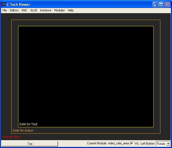
The VideoOutput Format changes the safe areas in the viewer window to match the default width and height values for the selected video format.
The Visible toggle turns the safe area display on and off. This toggle should always be off when making the actual video so the safe areas are not recorded.
The Move to Back toggle will put the safe area display behind any graphics in the viewer.
The Transparency slider changes the opacity of the safe area mask.
The Mask toggle turns the safe area masks on and off. The mask is a visual tool to help visualize which graphics fall into which safe area.
The Mask Text Area toggle turns the masking surrounding the text area on or off.
Mask Color alters the color of the masking.
The Lines toggle turns the lines defining the safe areas on and off.
The Labels toggle turns the labels defining the safe areas on and off.
The Action Border Color button selects the color of the action border.
The Text Border Color button selects the color of the text border.
Selecting Set viewer Res. sets the resolution of the viewer to the default for the video format that has been selected.
If the Preserve Width toggle is selected when the Set viewer Res. toggle is chosen, the current resolution width of the viewer will be maintained while the resolution height of the viewer will be based upon the appropriate ratio for the video format that has been selected.
If the Preserve Width toggle is unselected the Double Res toggle can be selected. The Double Res toggle will double the resolution of the viewer, while keeping the appropriate width-height ratio for the video format that has been selected. This should only be used while using the Screen Renderer output of output_images with the 4x4 anti-aliasing option.
The Update viewer button will set the viewer to the correct width and height if the Set viewer Res toggle has been selected.
advector
The advector module combines streamlines capability and a tool for sequential positioning of glyphs along the streamlines trajectory to simulate advection of weightless particles through a vector field (for example, a fluid flow simulation such as modflow). The result is an animation of particle motion, with the particles represented as any EVS geometry (such as a jet or a sphere). The glyphs can scale, deflect or deform according to the velocity vector it passes. At least one of the nodal data components input to advector must be a vector. The direction of travel of streamlines can be specified to be forwards (toward high vector magnitudes) or backwards (toward low vector magnitudes) with respect to the vector field. The input glyphs travel along streamlines (not necessarily visible in the viewer) which are produced by integrating a velocity field using the Runge-Kutte method of specified order with adaptive time steps.
Module Input Ports
- Z Scale [Number] Accepts Z Scale (vertical exaggeration).
- Input Field [Field] Accepts a field with vector data.
- Input Starting Locations [Field] Accepts a data field.
- Input Glyph [Field] Accepts a field representing the glyphs
Module Output Ports
- Output Field [Field] Outputs the glyphs
- Output Streamlines [Field] Outputs the streamlines field
- Output Glyph [Renderable]: Outputs the glyphs to the viewer.
- Output Streamlines Object [Renderable]: Outputs the streamlines to the viewer.
modpath_advector
The modpath_advector module combines MODPATH capability and a tool for sequential positioning of glyphs along the MODPATH lines trajectory to simulate advection of weightless particles through a vector field. The result is an animation of particle motion, with the particles represented as any EVS geometry (such as a jet or a sphere). The glyphs can scale, deflect or deform according to the velocity vector it passes. The direction of travel of streamlines can be specified to be forwards (toward high vector magnitudes) or backwards (toward low vector magnitudes) with respect to the vector field. The input glyphs travel along streamlines (not necessarily visible in the viewer) which are produced by integrating a velocity field using the Runge-Kutte method of specified order with adaptive time steps.
Module Input Ports
- Z Scale [Number] Accepts Z Scale (vertical exaggeration).
- Input Field [Field] Accepts a field with vector data.
- Input Starting Locations [Field] Accepts a data field.
- Input Glyph [Field] Accepts a field representing the glyphs
Module Output Ports
- Output Field [Field] Outputs the glyphs
- Output Streamlines [Field] Outputs the streamlines field
- Output Glyph [Renderable]: Outputs the glyphs to the viewer.
- Output Streamlines Object [Renderable]: Outputs the streamlines to the viewer.
read symbols
The read symbols module creates symbolic representations of different borehole identifiers based on a set of user defined parameters. The symbols are displayed at the top of the each borehole based on its x,y & z coordinates. A sample file with 48 predefined symbols is included, but it can be customized to produce special symbols.
Each symbol is made up of three components. The first shape is a fixed polygon with an outline. The thickness of the outline is selectable (via the control panel). A second polygon, which overlaps the first and has the same number of sides, has selectable minimum and maximum radial values (via the .SYM file). The third component is made up of a user defined set of lines (0 gives no lines). Each polygon has the same number of faces as defined in the #face parameter in the .SYM file. The area created by the difference between the Rmin value and the Rmax value is solid.
Module Input Ports
- Z Scale [Number] Accepts Z Scale (vertical exaggeration) from other modulesInput Geologic Field [Field] Accepts a data field from gridding and horizons to krige data into geologic layers.
- Filename [String / minor] Allows the sharing of file names between similar modules.
Module Output Ports
- Filename [String / minor] Allows the sharing of file names between similar modules.
- Sample Symbols [Renderable]: Outputs to the viewer
EVS.SYM file:
The following is a listing of the file evs.sym in evs\data\special. This file can be customized to produce other symbols.
# rmin rmax lmin lmax #face #line bw rot lrot rvrs name
48
1 0. 1 1 1 12 0 1 0 0 0 solid fill circle
2 0. .7 .7 1.2 12 4 1 0 0 0 solid fill circle w/ line
3 .8 1 1 1 12 0 1 0 0 0 circle ring
4 .4 1 1 1 12 0 1 0 0 0 fat circle ring
5 .0 .4 1 1 12 4 1 0 0 0 circle ring w/lines
6 .8 .7 .7 1.2 12 4 1 0 0 0 circle ring w/lines
7 .4 1 1 1 4 0 1 0 0 0 fat square box
8 .8 1 1 1 4 0 1 45 0 0 thin square box
9 .0 1 1 1 4 0 1 45 0 0 solid square box
10 .0 .7 .7 1.2 12 4 2 30 -30 0 half moon bk top w/line
11 .0 .7 .7 1.2 12 4 2 300 -300 0 half moon bk rt w/line
12 .0 .7 .7 1.2 12 4 2 210 -210 0 half moon bk bot w/line
13 .0 .7 .7 1.2 12 4 4 30 -30 0 qrtr moon bk ul w/line
14 .0 .7 .7 1.2 12 4 4 120 -120 0 qrtr moon bk ur w/line
15 .8 .7 0 1.2 12 4 1 0 0 0 open bulls-eye
16 .0 .7 .7 1.2 12 4 2 120 -120 0 half moon bk lft w/line
17 .0 1 1 1. 3 0 1 30 0 0 solid black triangle
18 .8 .7 .7 1.2 3 3 1 90 0 0 hollow blk triangle w/line
19 .0 1 1 1. 3 0 1 90 0 0 solid black triangle
20 .8 .7 .7 1.2 4 4 1 0 0 0 diamond w/line
21 .8 1 1 1. 4 0 1 0 0 0 diamond
22 .0 .7 .7 1.2 4 4 1 0 0 0 solid diamond w/line
23 .0 .7 .7 1.2 6 6 4 0 0 0 hex moon bk ul w/line
24 .0 .7 .7 1.2 6 6 4 180 0 0 hex moon bk ul w/line
25 0. 1 1 1 12 0 1 0 0 1 solid fill circle
26 0. .7 .7 1.2 12 4 1 0 0 1 solid fill circle w/ line
27 .8 1 1 1 12 0 1 0 0 1 circle ring
28 .4 1 1 1 12 0 1 0 0 1 fat circle ring
29 .0 .4 1 1 12 4 1 0 0 1 circle ring w/lines
30 .8 .7 .7 1.2 12 4 1 0 0 1 circle ring w/lines
31 .4 1 1 1 4 0 1 0 0 1 fat square box
32 .8 1 1 1 4 0 1 45 0 1 thin square box
33 .0 1 1 1 4 0 1 45 0 1 solid square box
34 .0 .7 .7 1.2 12 4 2 30 -30 1 half moon bk top w/line
35 .0 .7 .7 1.2 12 4 2 300 -300 1 half moon bk rt w/line
36 .0 .7 .7 1.2 12 4 2 210 -210 1 half moon bk bot w/line
37 .0 .7 .7 1.2 12 4 4 30 -30 1 qrtr moon bk ul w/line
38 .0 .7 .7 1.2 12 4 4 120 -120 1 qrtr moon bk ur w/line
39 .8 .7 0 1.2 12 4 1 0 0 1 open bulls-eye
40 .0 .7 .7 1.2 12 4 2 120 -120 1 half moon bk lft w/line
41 .0 1 1 1. 3 0 1 30 0 1 solid black triangle
42 .8 .7 .7 1.2 3 3 1 90 0 1 hollow blk triangle w/line
43 .0 1 1 1. 3 0 1 90 0 1 solid black triangle
44 .8 .7 .7 1.2 4 4 1 0 0 1 diamond w/line
45 .8 1 1 1. 4 0 1 0 0 1 diamond
46 .0 .7 .7 1.2 4 4 1 0 0 1 solid diamond w/line
47 .0 .7 .7 1.2 6 6 4 0 0 1 hex moon bk ul w/line
48 .0 .7 .7 1.2 6 6 4 180 0 1 hex moon bk ul w/line
sym #
Use to number(label) each symbols algorithm. This is the same
number used in the last column of the APDV data file.
Rmin, Rmax, Lmin, and Lmax
These values determine the size of the three possible shapes used to create each symbol. The center point is at 0.0 and the outer edge of the polygons is at 1.0. The x/y lines can start at the center(0.0) or at any other position within the polygon. They can also be extended beyond 1.0 to a position of 1.7.
Rmin
Sets the minimum radius of the inside of the second polygon. With a setting of 0.0 the inside is fully minimized thus creating a solid polygon from the center out to Rmax. A setting of 0.8 will create a solid polygon, with an empty center, out to Rmax.
Rmax
Sets the maximum radius of the outside of the second polygon. A setting of 1.0, places the outside edge directly over the outside edge of the first, fixed polygon. A setting of 0.2 and a Rmin setting of 0.0 creates a small solid polygon centered in the middle of the first polygon.
Lmin
Sets the starting point for the x/y lines. 0.0 starts the lines from the center of the polygons. 1.0 starts the lines at the outer edge of the polygons.
Lmax
Determines how far the lines will extend from Lmin. If Lmax and Lmin equal 1.0 then no lines will be displayed. If Lmin is 0.0 and Lmax is 1.7 the lines will extend from the center past the outer edge of the polygons.
#face
This value determines the number of faces both polygons will display. A value of 12 displays a convincing circle.
#line
This value determines the number of lines.
bw
This parameter allows you to divide the second polygon into alternating light/dark solids with a x/y axis.
Valid values are 1, 2 and 4.
1 = full solid
2 = half solid
3 = alternating quarter solids
rot
Sets the rotation of the symbol in degrees.
lrot
Sets the rotation of the lines relative to the symbol in degrees.
rvrs
Use this parameter to reverse the symbols colors. A value of 0 is normally used but a value of 1 will reverse the colors.
name
an optional description of each symbol. This is only used for reference within the SYM file.
Sample Module Networks
The sample network shown below reads a GEO formatted data file, and a SYM formatted algorithm file. The output is displayed by the geometry viewer.
Symbols
|
|
EVS viewer
A test geology file is included in the evs\special directory called TEST_SYM.GEO. It displays all 48 of the default symobls defined in the file shown above. The symbols are oriented starting at the lower left hand corner and going left to right and bottom to top.
create_spheroid
This module is deprecated and replaced by place_glyph
The create_spheroid module produces a 2D circular disc or 3D spheroidal or ellipsoidal grid that can be used for any purpose, however the primary application is as starting points for 3d streamlines or advector.
Module Input Ports
- Input Field [Field] Accepts a field to extract its extent
Module Output Ports
- Output Field [Field / Minor] Outputs the surface
- Surface [Renderable]: Outputs to the viewer
advect_surface
The advect_surface module combines surface streamlines capability and a tool for sequential positioning of glyphs along the streamlines trajectory to simulate advection of particles down a surface. The result is an animation of particle motion, with the particles represented as any EVS geometry (such as a jet or a sphere). The glyphs can scale, deflect or deform according to the velocity vector. The direction of travel of streamlines can be specified to be downhill or uphill (for the slope case). The input glyphs travel along streamlines (not necessarily visible in the viewer) which are produced by integrating a velocity field using the Runge-Kutte method of specified order with adaptive time steps.
The advect_surface module is used to produce streamlines and particle animations on any surface based on its slopes. The direction of travel of streamlines can be specified to be downhill or uphill for the slope case. A physics simulation option is also available which employs a full physics simulation including friction and gravity terms to compute streamlines on the surface.
Module Input Ports
- Z Scale [Number] Accepts Z Scale (vertical exaggeration).
- Input Field [Field] Accepts a field with vector data.
- Input Starting Locations [Field] Accepts a data field.
- Input Glyph [Field] Accepts a field representing the glyphs
Module Output Ports
- Output Field [Field] Outputs the glyphs
- Output Streamlines [Field] Outputs the streamlines field
- Output Glyph [Renderable]: Outputs the glyphs to the viewer.
- Output Streamlines Object [Renderable]: Outputs the streamlines to the viewer.
fence_geology
The fence_geology module uses data in specially formatted .geo files to model the surfaces of geologic layers in vertical planes, or cross sections. Fence Geology essentially creates layers of quadrilateral (4 node) elements (in a vertical plane) in which each node (and element) is assigned to an individual geologic layer. The output of fence_geology is a data field, consisting of a 2D line with each layers elevation as nodal data elements, that can be sent to the krig_fence and horizons to 3d modules where the quadrilateral elements are connected to the element nodes in adjacent geologic surfaces to create layers along the fence.
Module Input Ports
- Input Filename [String] Receives the filename from other modules.
- Input Line [Field ] Allows the user to import a line (path) to which all data will be kriged.
Module Output Ports
- Geologic legend Information [Geology legend] Supplies the geologic material information for the legend module.
- Output Line [Field] Connects to krig_fence
- Filename [String / minor] Outputs a string containing the file name and path. This can be connected to other modules to share files.
file_output
The file_output module creates a formatted string based upon the values passed to it. This string is then written to the selected ascii text file. Certain modules such as 3d estimation, krig_2d, and krig_fence output a formatted string for just this purpose.
adaptive_indicator_krig
adaptive_indicator_krig is an alternative geologic modeling concept that uses geostatistics to assign each cell’s lithologic material as defined in a pregeology (.pgf) file, to cells in a 3D volumetric grid.
There are two methods of lithology assignment:
- Nearest Neighbor is a quick method that merely finds the nearest lithology sample interval among all of your data and assigns that material. It is very fast, but generally should not be used for your final work.
- Kriging provides the rigorous probabilistic approach to geologic indicator kriging. The probability for each material is computed for each cell center of your grid. The material with the highest probability is assigned to the cell. All of the individual material probabilities are provided as additional cell data components. This will allow you to identify regions where the material assignment is somewhat ambiguous. Needless to say, this approach is much slower (especially with many materials), but often yields superior results and interesting insights.
adaptive_indicator_krig is an extension of the technology in lithologic modeling for several reasons:
- Material assignments are done on a nodal versus cell basis providing additional inherent resolution
- Gridding is handled by outside modules. This allows for assigning material data based on a PGF file after kriging analyte (e.g. chemistry) or other parameter data with 3d estimation.
- Though it does not provide material boundaries that are as smooth as gridding and horizons, it does provide much smoother interfaces than lithologic modeling’s Lego-like material structures.
There are two fundamental differences between lithologic modeling and adaptive_indicator_krig
- Geology / Grid input:
- lithologic modeling expects input from modules like gridding and horizons (which is a set of surfaces) and it builds you grid for you just as 3d estimation does.
- adaptive_indicator_krig is more like the “Kriging to an external grid” option in 3d estimation. You need to create the 3D grid (which doesn’t need to have any data) that it will use. It will take that grid as a starting point for material assignments and later smoothing.
- Lithologic Material Assignment
- lithologic modeling assigns whole cells to cell sets and sets CELL data which is Material_ID.
- adaptive_indicator_krig takes the external grid and further refines it by splitting whole cells along all boundaries between two or more materials to create smoother interfaces.
Module Input Ports
- Input Field [Field] Accepts a data from 3d estimation, horizons to 3d or other modules that have already created a grid containing volumetric cells. If the input field has data such as concentrations, it will be included in the output.
- Filename [String / minor] Allows the sharing of file names between similar modules.
- Refine Distance [Number] Accepts the distance used to discretize the lithologic intervals into points used in kriging.
Module Output Ports
- Geologic legend Information [Geology legend] Supplies the geologic material information for the legend module.
- Output Field [Field] Contains nodal data and a refined grid representing geologic materials..
- Filename [String / minor] Outputs a string containing the file name and path. This can be connected to other modules to share files.
- Refine Distance [Number] Outputs the distance used to discretize the lithologic intervals into points used in kriging or displayed in post_samples as spheres.
Properties and Parameters
The Properties window is arranged in the following groups of parameters:
- Grid Settings: control the grid type, position and resolution
- Krig Settings: control the estimation methods
- NOTE: Nearest Neighbor assigns the lithologic material cell data based on the nearest lithologic material (in anisotropic space) to your PGF borings. This is done based on the cell center (coordinates) and an enhanced refinement scheme for the PGF borings. In general Nearest Neighbor should not be used for final results
Advanced Variography Options:
It is far beyond the scope of our Help to attempt an advanced Geostatistics course. The terminology and variogram plotting style that we use is industry standard and we do so because we will not provide detailed technical support nor complete documentation on these features, which would effectively require a geostatistics textbook, in our help.
However, we have offered an online course on how to take advantage of the complex, directional anisotropic variography capabilities in adaptive_indicator_krig(which applies equally well to lithologic modeling and 3d estimation), and that course is available as a recorded video class. This class is focused on the mechanics of how to employ and refine the variogram anisotropy with respect to your data and the physics of your project such as contaminated sediments in a river bottom. The variogram is displayed as an ellipsoid which can be distorted to represent the Primary and Secondary anisotropies and rotated to represent the Heading, Dip and Roll. Overall scale and translation are also provided as additional visual aids to compare the variogram to the data, though these do not affect the actual variogram.
We are not hiding this capability from you as the Anisotropic Variography Study folder of Earth Volumetric Studio Projects contains a number of sample applications which demonstrate exactly what is described above. However, we assure you that understanding how to apply this to your own projects will be quite daunting and really does require a number of prerequisites:
- A thorough explanation of these complex applications
- A reasonable background in Python and how to use Python in Studio
- An understanding of all of the variogram parameters and their impact on the estimation process on both theoretical datasets as well as real-world datasets.
This 3 hour course addresses this issues in detail.
krig_fence
krig_fence models parameter distributions within domains defined by the boundaries of the input data in 3D Fence sections which can “snake” around in the x-y plane and are parallel to the z-axis. krig_fence can also receive the geologic system modeled by Fence Geology. It creates a quadrilateral finite-element grid with kriged nodal values of any scalar property and its kriged confidence level, and outputs a geometry whose elements can be rendered to view the color scaled parameter distribution on the element surfaces. krig_fence provides several convenient options for pre- and post-processing the input parameter values, and allows the user to consider anisotropy in the medium containing the property.
Module Input Ports
- Filename [String / minor] Allows the sharing of file names between similar modules.
- Fence Geology Input [Field] Accepts a field from krig_fence containing geologic layers.
- Input External Data [Field / minor] Allows the user to import a field contain data. This data will be kriged to the grid instead of using file data.
Module Output Ports
- Filename [String / minor] Allows the sharing of file names between similar modules.
- Output Field [Field] Outputs a 3D data field which can be input to any of the Subsetting and Processing modules.
- Status Information [String / minor] Outputs a string containing module parameters. This is useful for connection to write evs field to document the settings used to create a grid.
fence_geology_map
The fence_geology_map module creates 3-dimensional fence diagram from the 1-dimensional line contours which follow your geology produced by fence_geology, to allow visualizations of the geologic layering of a system. It accomplishes this by creating a user specified distribution of nodes in the Z dimension between the top and bottom lines defining each geologic layer.
The number of nodes specified for the Z Resolution may be distributed (proportionately) over the geologic layers in a manner that is approximately proportional to the fractional thickness of each layer relative to the total thickness of the geologic domain. In this case, at least three layers of nodes (2 layers of elements) will be placed in each geologic layer.
Module Input Ports
- Input Geologic Field [Field] Accepts fence_geology output
Module Output Ports
- Output Field [Field] Outputs the field
application_notes
The application_notes has been deprecated and replaced by the Annotation’s “Notes”
texture_colors
This is a deprecated module
texture_colors functionality has been incorporated into all modules. On the Home tab, you have the Render Method selector where you can choose to use Vertex RGB coloring or Textures.
texture_wave
The texture_wave module utilizes transparency and texture mapping similar to texture_colors and illuminated_lines technology to create an animated effect. However, unlike illuminated_lines, this module works with both OpenGL and Software Rendering.
texture_wave has a single input port that accepts the grid with nodal data that you want to color with this technique. This would normally be tubes or streamribbons.
The Phase is the parameter that changes during the animation loop.
Number of Steps: determines the number of steps in the animation.
Texture Resolution is the internal resolution of the image used for texture-coloring.
Min Amplitude is the minimum opacity of the objects.
Max Amplitude is the maximum opacity of the objects.
Contrast affects the contrast (similar to color saturation).
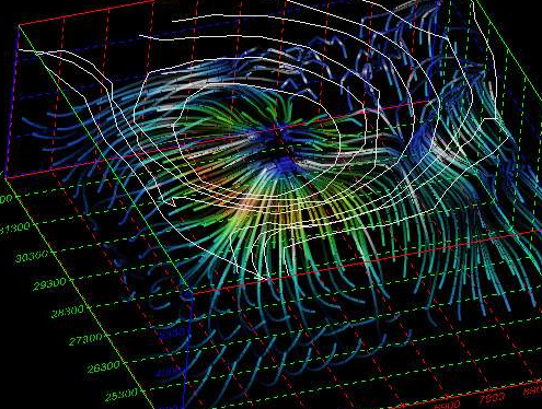
In the image below, we used streamlines which are passed to tubes, which are then connected to texture_wave. The transparency, colors, and animation effects on the tubes is all performed by texture_wave.
The viewer window is shown below.
illuminated_lines
Display of Illuminated Lines using texture mapped illumination model on polylines with line halo and animation effects.
Prerequisites
This module requires OpenGL rendering to be selected. This module utilizes special OpenGL calls to implement the illuminated line technique. If this module is used with another renderer, such as the software renderer or the output_images module (not set to Automatic), lines will be drawn in the default mode with illuminated line features disabled.
This module requires the input mesh to contain one Polyline cell set. Any other type of cell set will be rejected, and any additional cell sets will be ignored. Any scalar node data may be present, or none for purely geometric display.
Animation Effects
Ramped/Stepped This choice selects the style of effect variation. Stair creates a linearly increasing or decreasing value, while step makes a binary chop effect. In Ramped mode, the blending can be selected to start small then get big, or the reverse or both. The values are down, up, up&down respectively. Stepped causes abrupt changes in effect.
AnimatedLength This slider sets the length of the effect along the polyline.
AnimationSpacing This slider sets the spacing between effects along the line.
ModulateOpacity In this mode the line segment varies in transparency from completely transparent to opaque.
ModulateWidth In this mode the line width is varied between 1 (very thin) to fat, based on the effect modes and shape controls.
Reverse Effect As the animation effect is applied between two zones, such as the dash and the space between the dash, this toggle reverses the area where the effect is applied.
Halo Parameters
Halo Width The width control for the halo effect defines the size of the transparent mask region added to the edge of each line. A value of zero turns off the halo effect.
Illuminated Lines Shading Model
AmbientLighting This value provides a base shadow value, a constant added to all shading values.
DiffuseLighting Pure diffuse reflection term, amount of shading dependent on light angle
SpecularHighlights Amount of specular reflection hi-lights based on light and viewer angle
Specular Focus Tightness of specular reflection, low values are dull, wide reflections, high values are small spot reflections.
Line Width Controls line width. Normal 1-pixel lines are 1, can be increased in whole increments. Wide lines are drawn in 2D screen space, not full 3D ribbons. If you want full ribbons, use streamline module ribbon mode.
Line Opacity Variable transparency of all lines. A value of 1.0 is fully opaque, while a value of zero makes lines invisible.
DataColor Blending If node data is present, this controls the relative mix of data color and shading color. A value of zero sets full contribution of data color, while at 1.0 no data color is used and the line shade is dominated by illumination effects.
Smooth Shading This enables an additional interpolation mode for blended node data colors. In the off state, data is sampled once per line segment. When enabled, linear interpolation is used between end points of each segment. This can be helpful if large gradients are present on low resolution polylines.
Antialias This effect, sometimes called “smooth lines” blends the drawing of lines to create a smooth effect, reducing the effects of “jaggies” at pixel resolution.
Sort Trans This mode assists visual quality when transparency or antialiasing modes are used, helping to reduce artifacts caused by non-depth sorted line crossings.