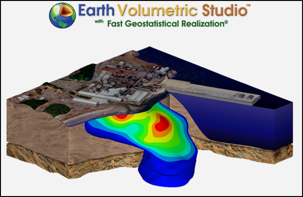
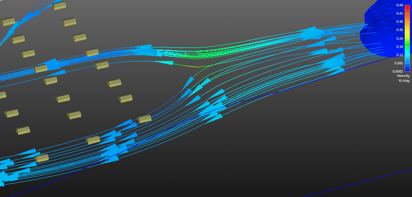
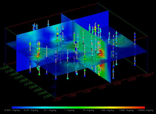
C Tech’s Earth Volumetric Studio is the world’s leading three-dimensional volumetric Earth Science software system developed to address the needs of all Earth science disciplines. Studio is the culmination of C Tech’s 30+ years of 3D modeling development, building upon the developments of legacy software EVS-Pro, MVS and EnterVol. Studio’s customizable toolkit is targeted at geologists, environmental engineers, geochemists, geophysicists, mining engineers, civil engineers and oceanic scientists. Whether your project is a corner gas station with leaking underground fuel tanks, a geophysics survey of a large earthen dam combining 3D resistivity and magnetics data, or modeling of salt domes and solution mined caverns for the U.S. Strategic Petroleum Reserves, C Tech’s Earth Volumetric Studio has the speed and functionality to address your most challenging tasks. Our software is used by organizations worldwide to analyze all types of analyte and geophysical data in any environment (e.g. soil, groundwater, surface water, air, etc.).
This section of the documentation provides a guide to the main components of the Earth Volumetric Studio (EVS) user interface. It is designed to help you understand the layout, functionality, and interaction between the different windows and tools that form the core of the application.
From the initial Startup Window to the detailed Properties panels and the powerful Viewer, these articles cover everything you need to know to navigate and manage your workspace effectively.
EVS Presentations (.EVSP) provide a single file deliverable which allows our customers to provide versions of their Earth Volumetric Studio (EVS) applications to their clients, who can then modify properties interactively.
For example, an EVS Presentation can allow your clients to:
Choose their own plume levels Change Z-Scale and/or Explode distance Move slices or cuts through the model Draw their own paths for (cross section) cross-sections This works by creating a restricted version of an EVS application, saved as an EVS Presentation (.evsp file).
Basic Training: Workbooks Overview
The Earth Volumetric Studio Environment 2D Estimation Exporting from Excel to C Tech File Formats 3D Data Requirements Overview Packaging Data into Applications Geostatistics Overview Visualization Fundamentals
Video Tutorials at ctech.com
The workbooks in this help cover only the most basic functionality. We offer two levels of training videos which can be accessed at ctech.com which provide more comprehensive training from a novice to an advanced user. We offer two levels of training videos in addition to the limited workbooks which are built-into the software help system (and are included online). The training videos include:
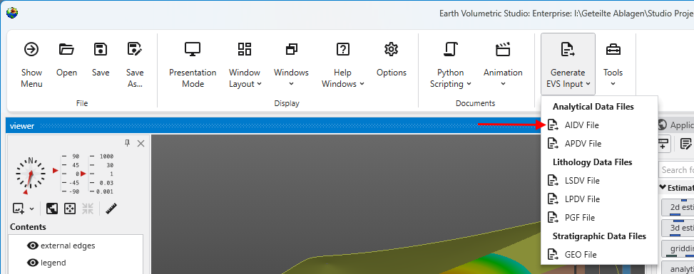
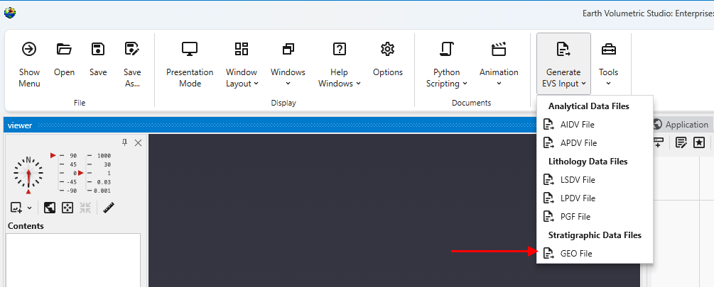
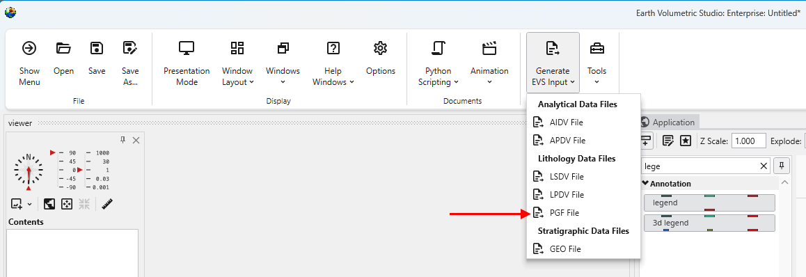
EVS Data Input & Output Formats
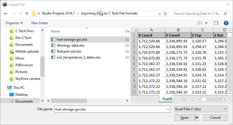
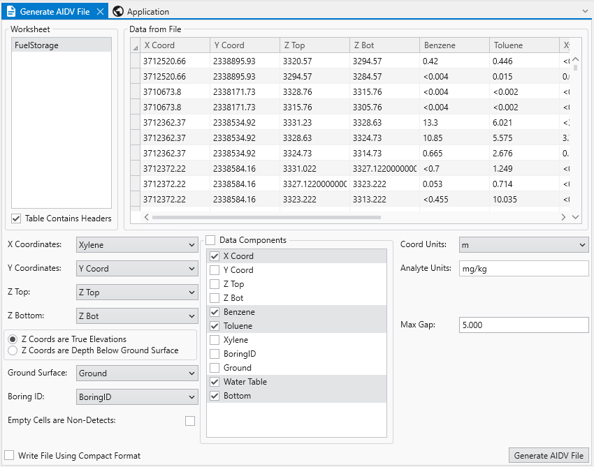
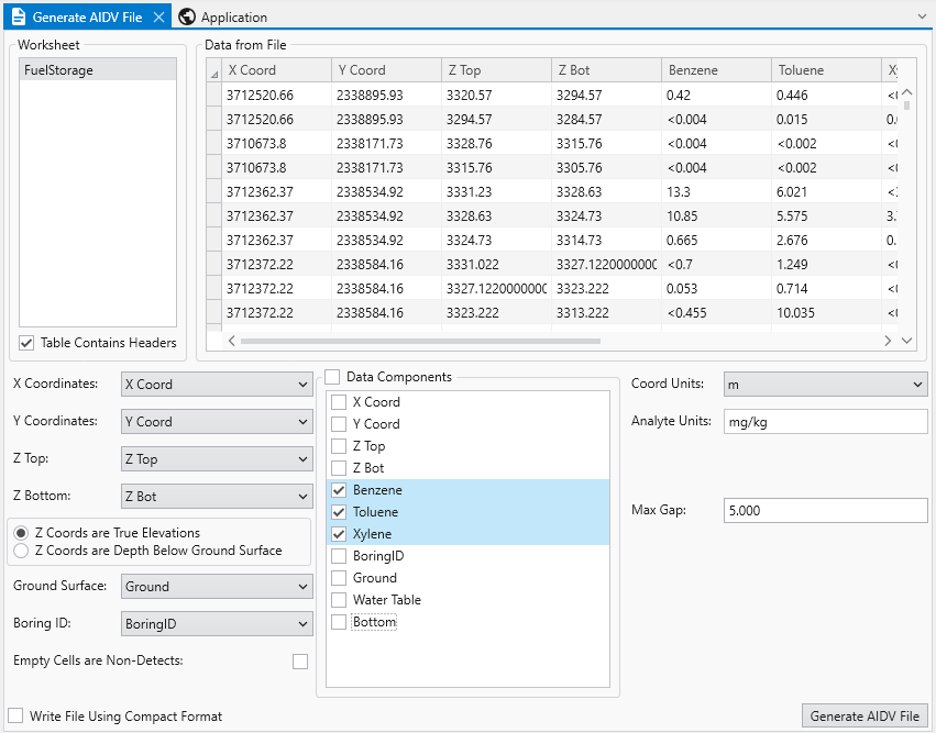
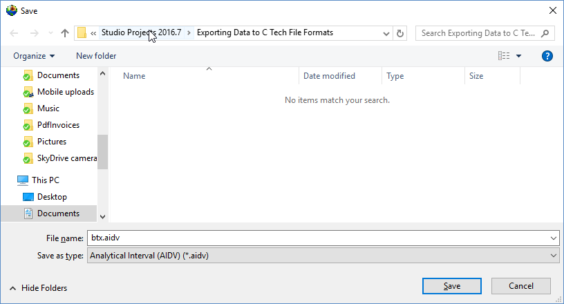
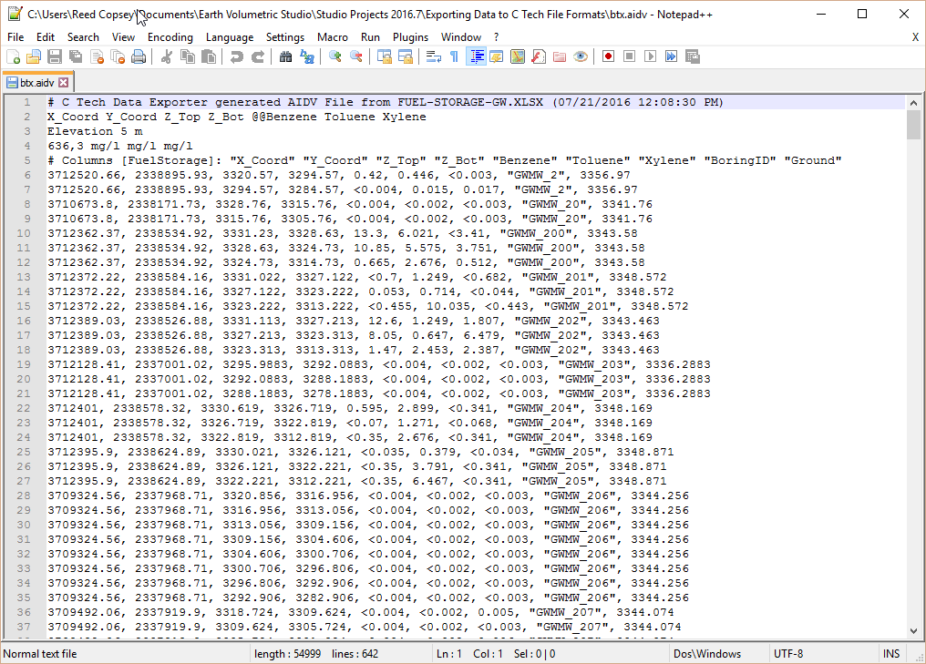
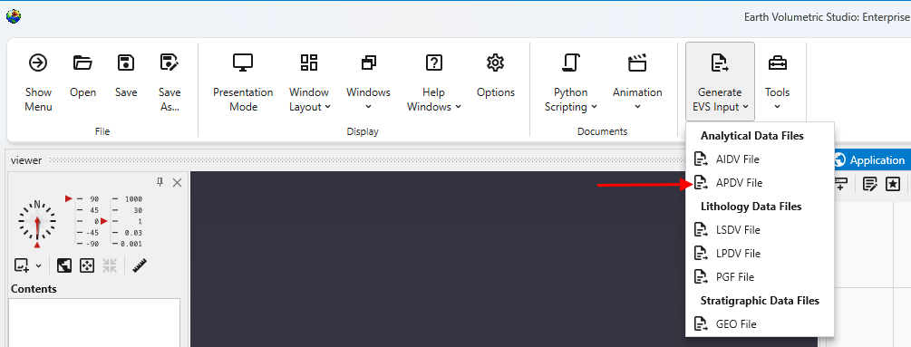
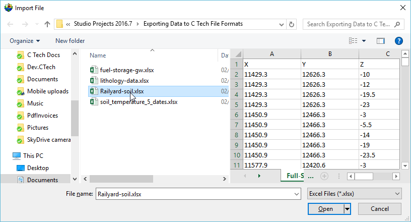
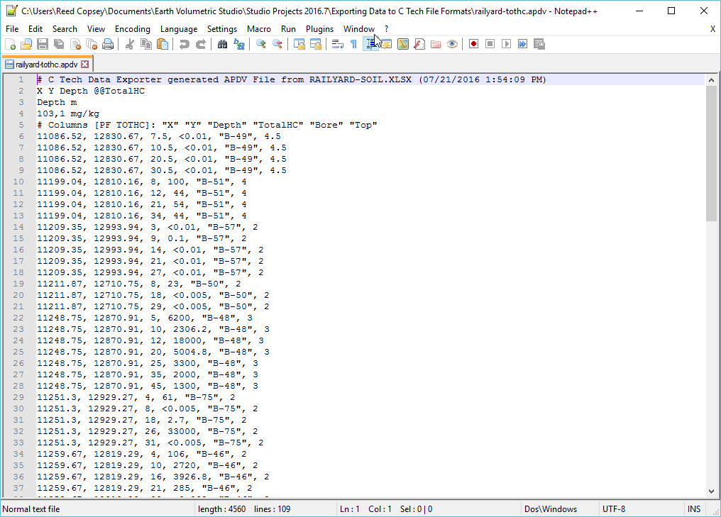
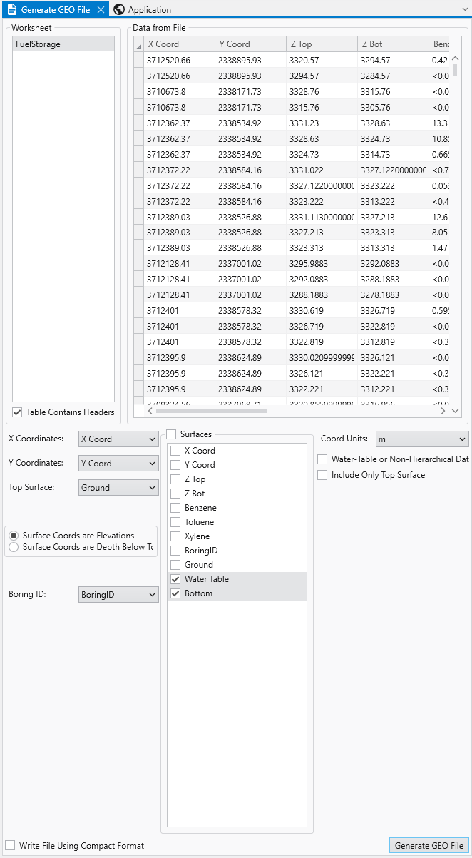
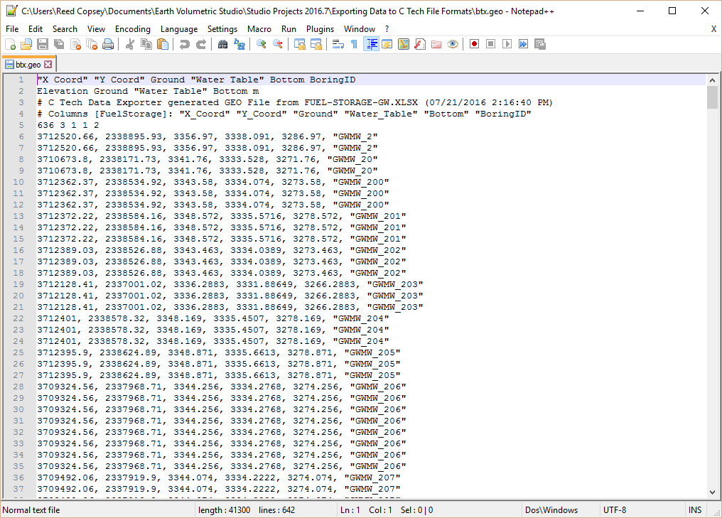
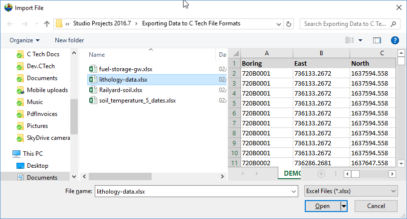
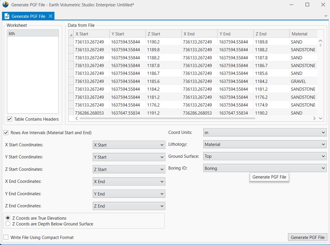
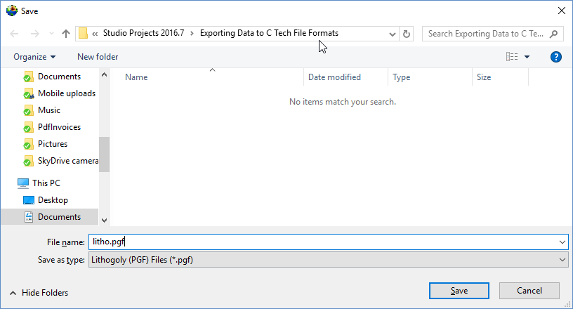
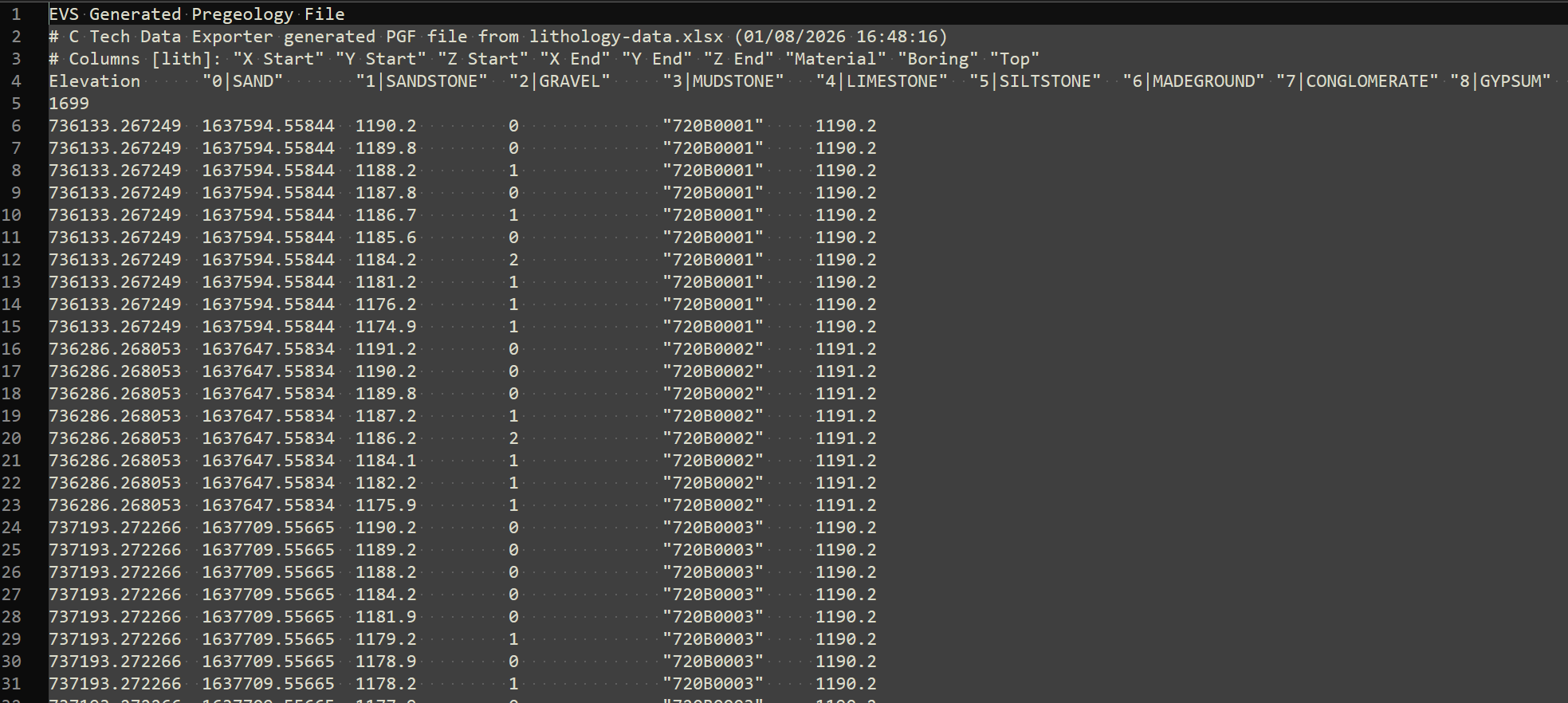
EVS Data Input & Output Formats Input EVS conducts most of its analysis using input data contained in a number of ASCII files. These files can generally be created using the Data Transformation Tools, which are on the Tools tab of EVS. These tools will create C Tech’s formats from from Microsoft Excel files.
Handling Non-Detects
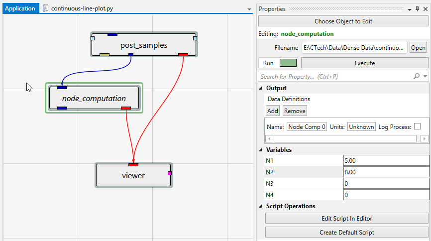
Handling Non-Detects It is important to understand how to properly handle samples that are classified as non-detects. A non-detect is an analytical sample where the concentration is deemed to be lower than could be detected using the method employed by the laboratory. Non-detects are accommodated in EVS for analysis and visualization using a few very important parameters that should be well understood and carefully considered. These parameters control the clipping non-detect handling in all of the EVS modules that read chemistry (.apdv, or .aidv) files. The affected modules are 3d estimation, krig_2d, post_samples, and file_statistics.
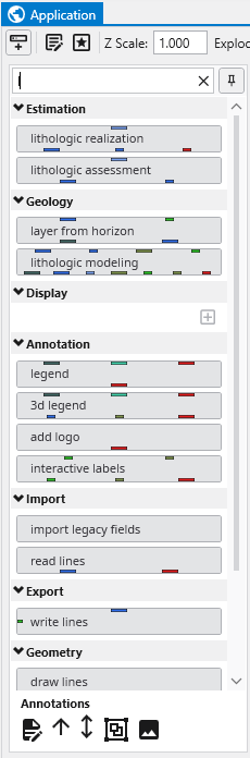
Module Libraries EVS modules can each be considered software applications that can be combined together by the user to form high level customized applications performing analysis and visualization. These modules have input and output ports and user interfaces.
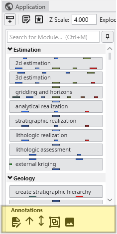
The library of module are grouped into the following categories:
Estimation modules take sparse data and map it to surface and volumetric grids Geology modules provide methods to create surfaces or 3D volumetric grids with lithology and stratigraphy assigned to groups of cells Display modules are focused on visualization functions Analysis modules provide quantification and statistical information Annotation modules allow you to add axes, titles and other references to your visualizations Subsetting modules extract a subset of your grids or data in order to perform boolean operations Proximity modules create new data which can be used to subset or assess proximity to surfaces, areas or lines. Processing modules act on your data Import modules read files that contain grids, data and/or archives Export modules write files that grids, data and/or archives Modeling modules are focused on functionality related to simulations and vector data Geometry modules create or act upon grids and geometric primitives Projection modules transform grids into other coordinates or dimensionality Image modules are focused on aerial photos or bitmap operations Time modules provide the ability to deal with time domain data Tools are a collection of modules to make life easier View modules are focused on visualization and output of results Legacy Module Naming
Command Line Automation
Automation of EVS Given an appropriate Enterprise license or Automation license, EVS can be run in a fully automated manner in two ways. The first is to use special command line flags to run the program, open applications, run scripts, and cleanly close when complete. The second is to use an external language and programming API to control EVS via custom written code.
Automating EVS via Custom Code
Reducing Complexity in Applications C Tech recommends avoiding overly large applications. There are numerous ways to reduce the number of modules and complexity of an application, including but not limited to:
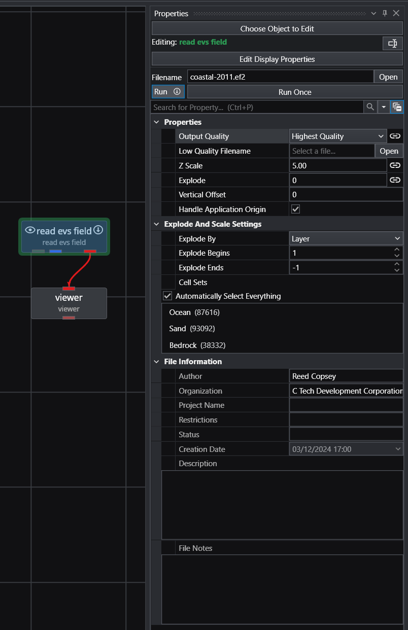
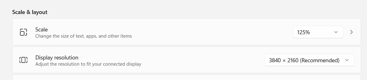
Once the grid and estimation is complete, save those results as an EF2 file. A single read evs field module can then (typically) replace 3 to 5 modules. If the complexity is there to address multiple analytes and/or threshold levels in a CTWS file, scripted sequences can often reduce the number of modules by a factor of 5 or more. Understanding Display Resolution and Scaling The usability of EVS is influenced by your display’s effective resolution, which is a combination of its native resolution (e.g., 4K) and the scaling setting in Windows (e.g., 150%).
Detailed instructions for installation and licensing of all license types are available here.
This section of the documentation provides a guide to the main components of the Earth Volumetric Studio (EVS) user interface. It is designed to help you understand the layout, functionality, and interaction between the different windows and tools that form the core of the application.
From the initial Startup Window to the detailed Properties panels and the powerful Viewer, these articles cover everything you need to know to navigate and manage your workspace effectively.
By familiarizing yourself with these components, you will be able to build, visualize, and analyze your projects more efficiently.
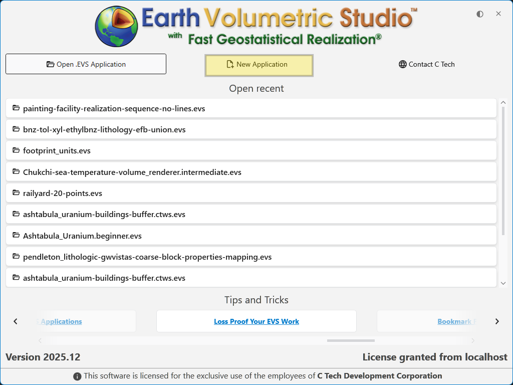
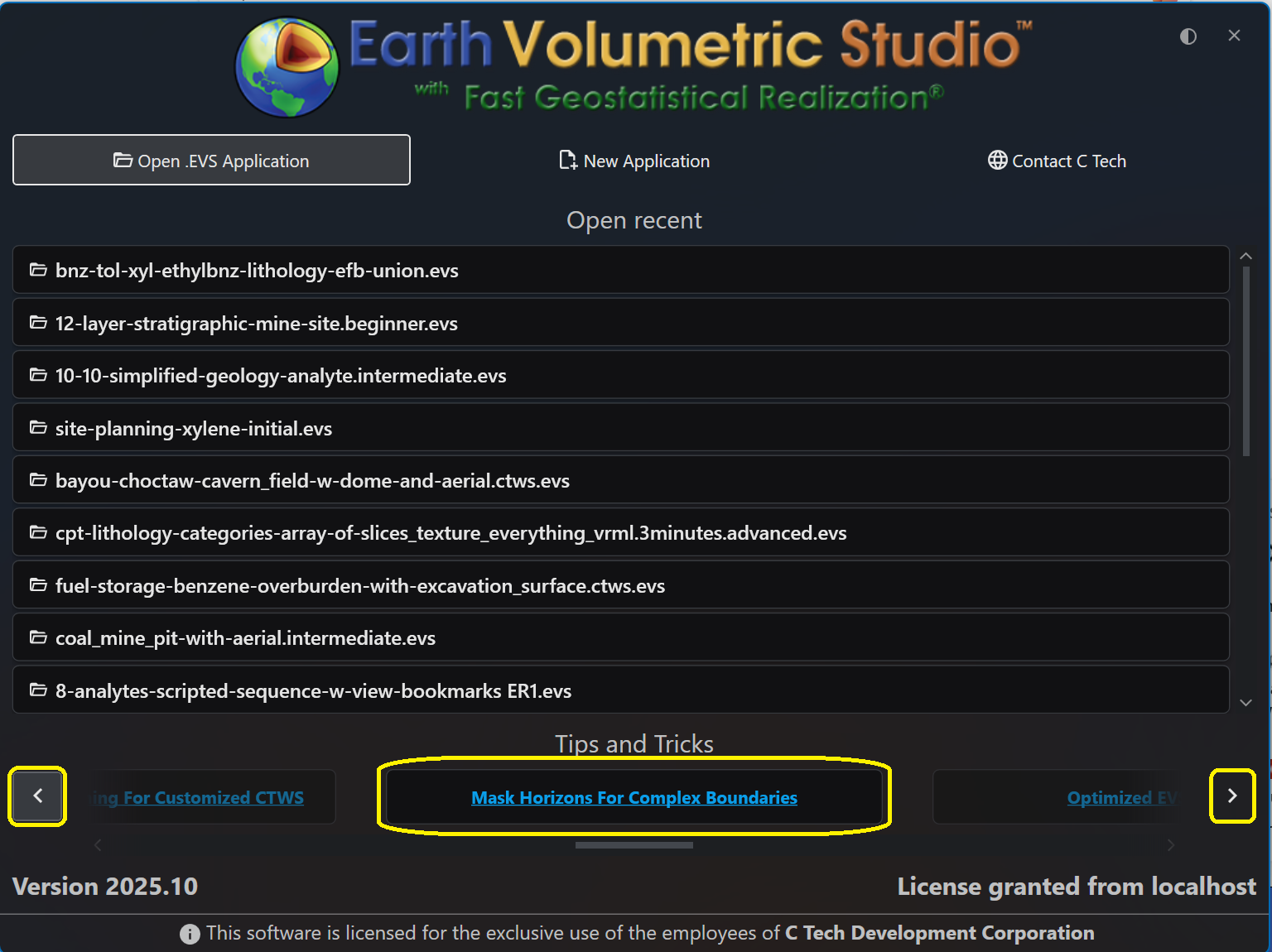
The Earth Volumetric Studio startup window is your launchpad for any project. From here, you can start with a clean slate by creating a new application, jump back into a previous project by opening an existing file, or access helpful resources.
Licensing and Version Information The bottom of the window shows you the current version of EVS as well as well as your license status.
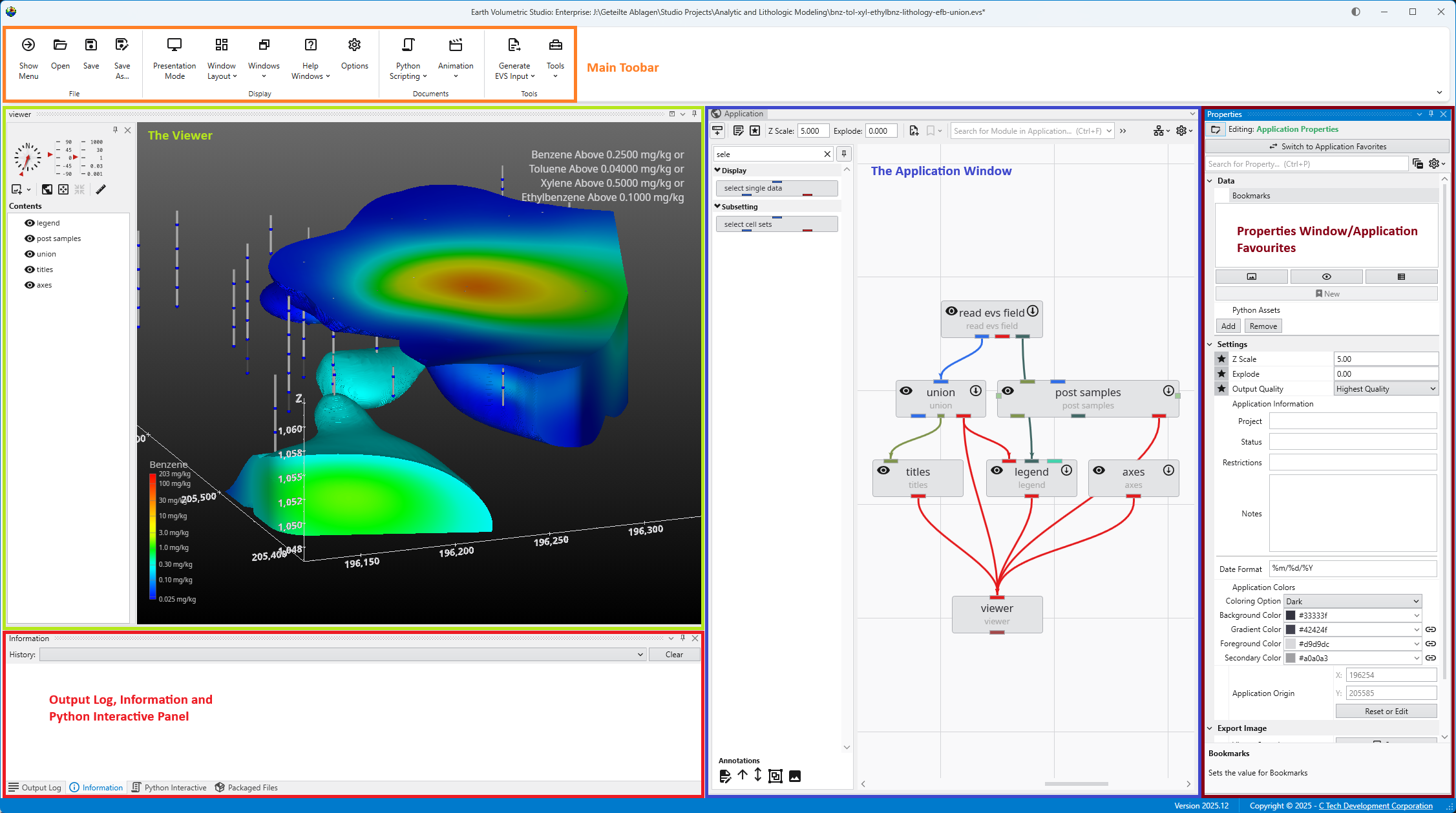
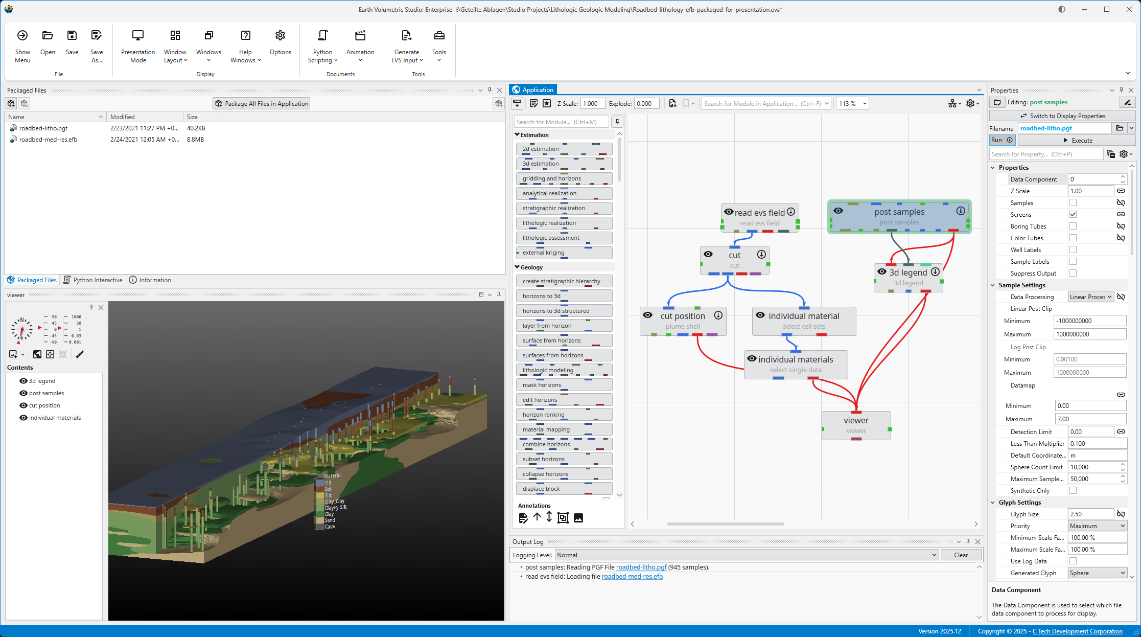
Getting Started with the EVS User Interface The main window is organized into five primary sections in the default layout configuration, each designed to provide a streamlined workflow for your data processing, visualization, and analysis needs. Most windows can be freely docked or undocked in any configuration and layouts can be loaded and saved.
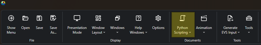
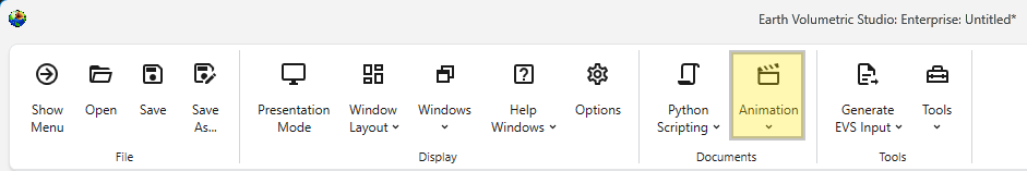
The Main Toolbar The Main Toolbar is the primary command bar in Earth Volumetric Studio, located at the top of the main application window. It provides streamlined access to the application’s most common features and functions. The toolbar is organized into logical sections: File, Display, Documents, and Tools, making it easier to locate and use the necessary commands for your projects.
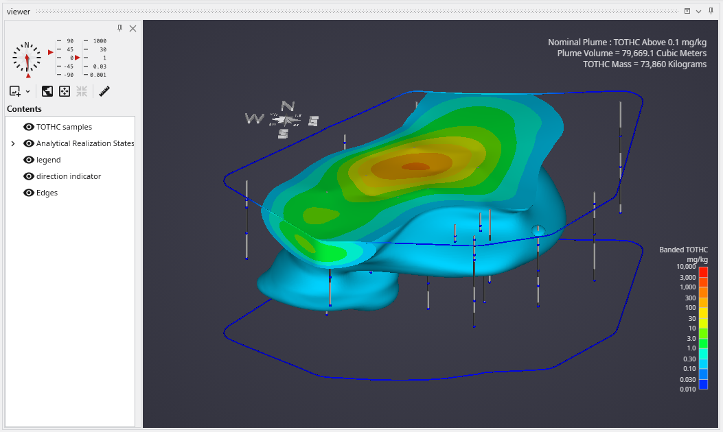
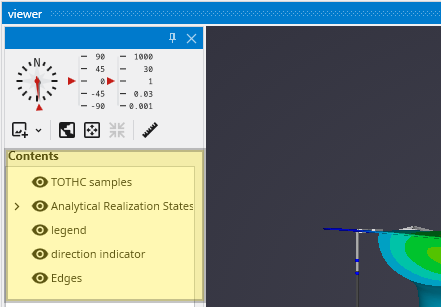
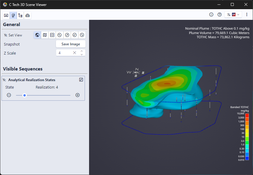
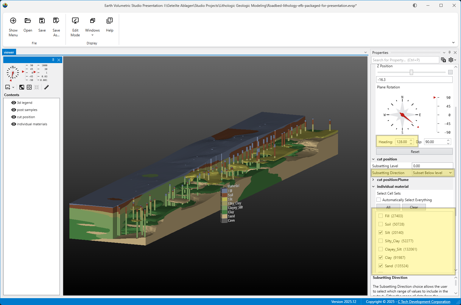
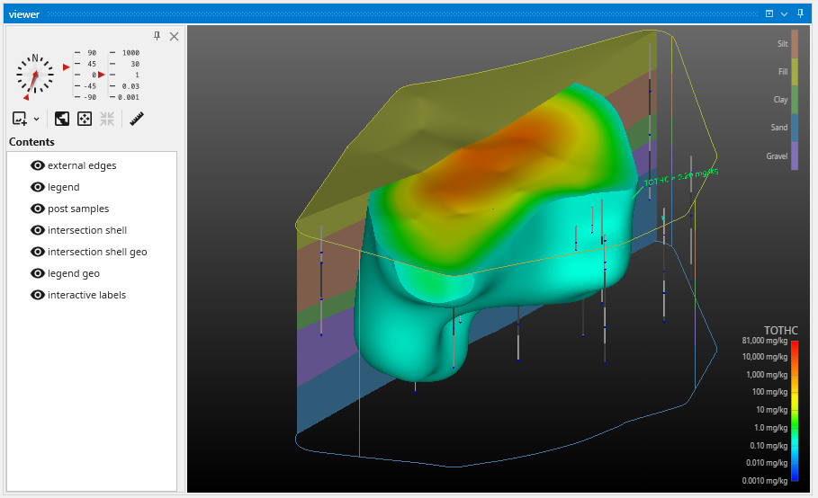
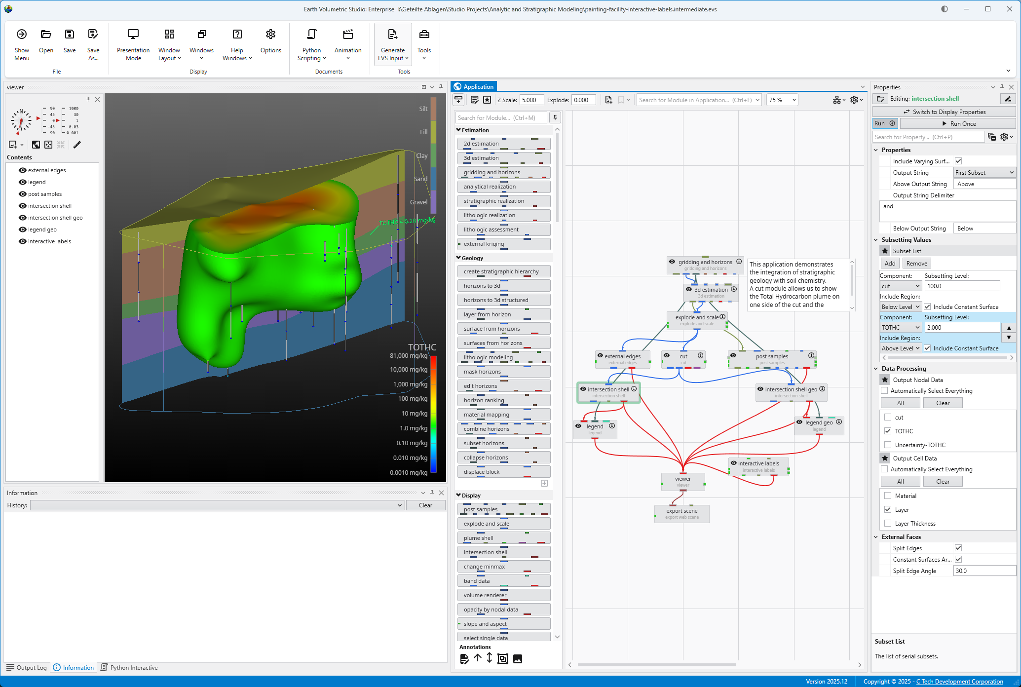
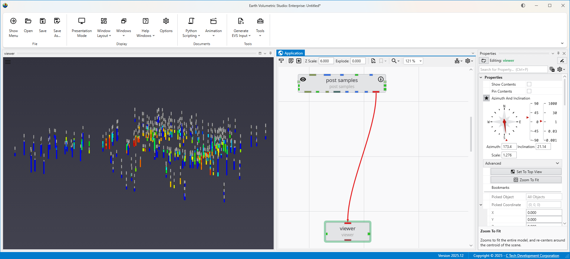
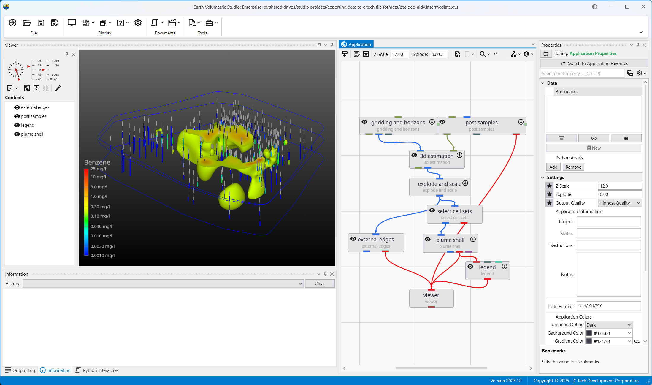
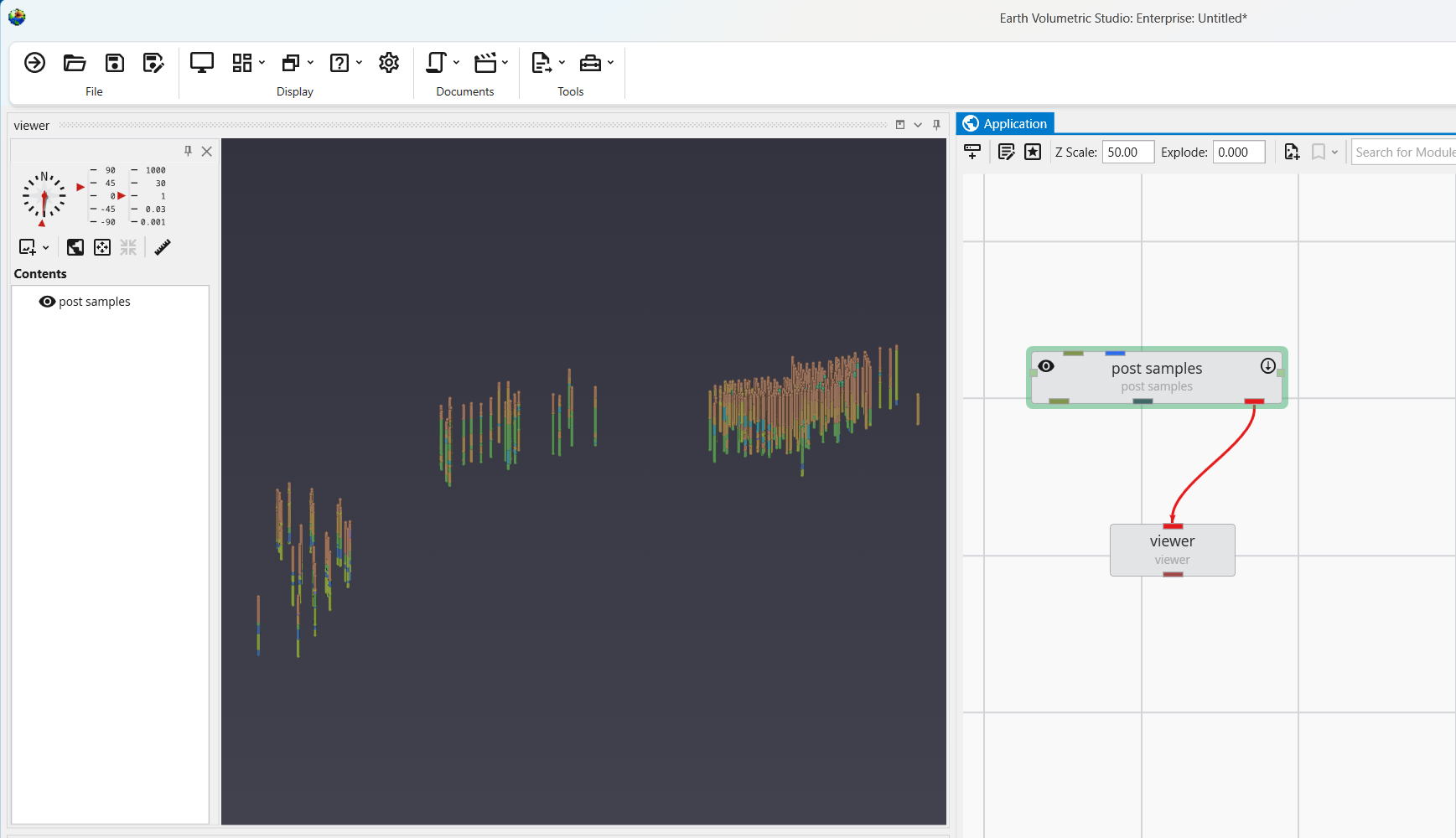
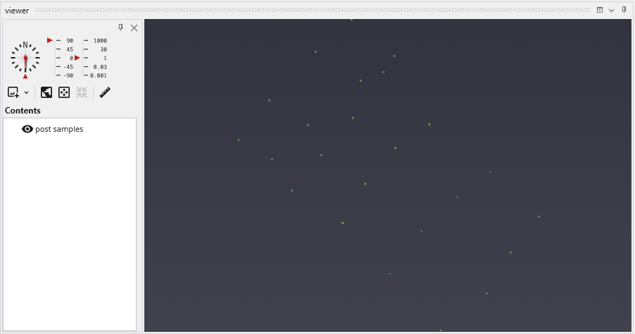
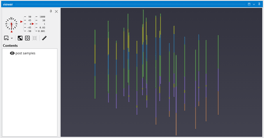
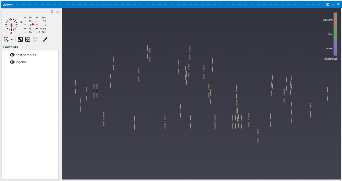
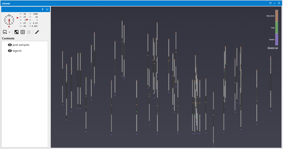
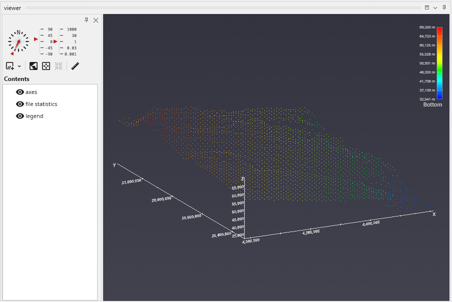
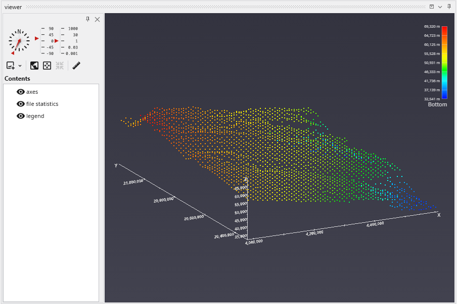
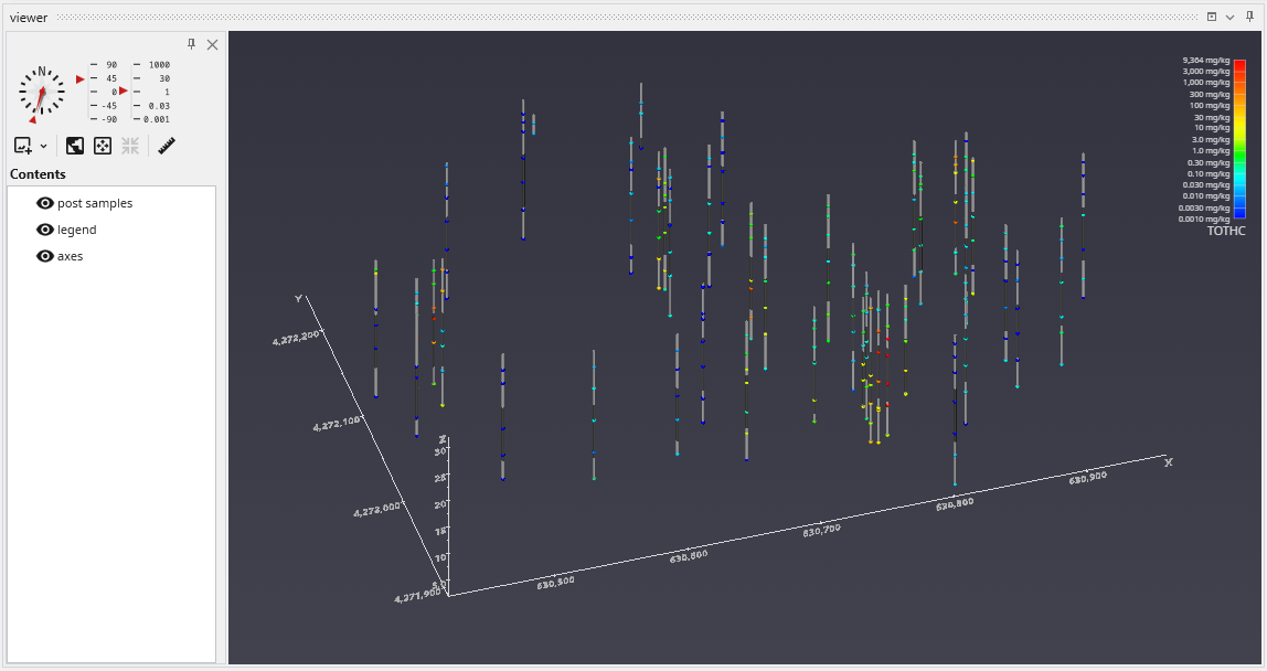
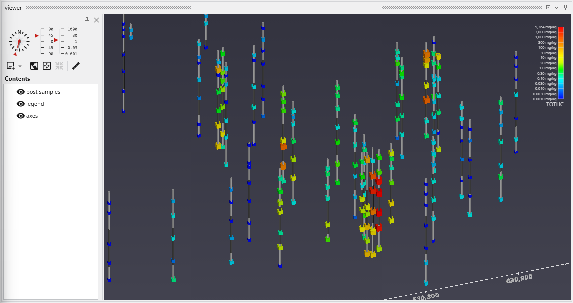
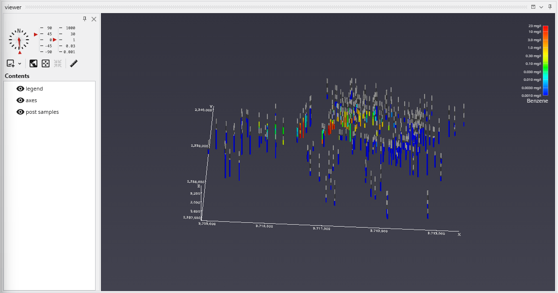
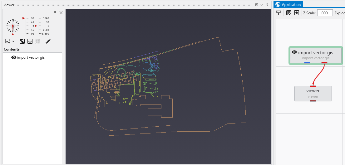
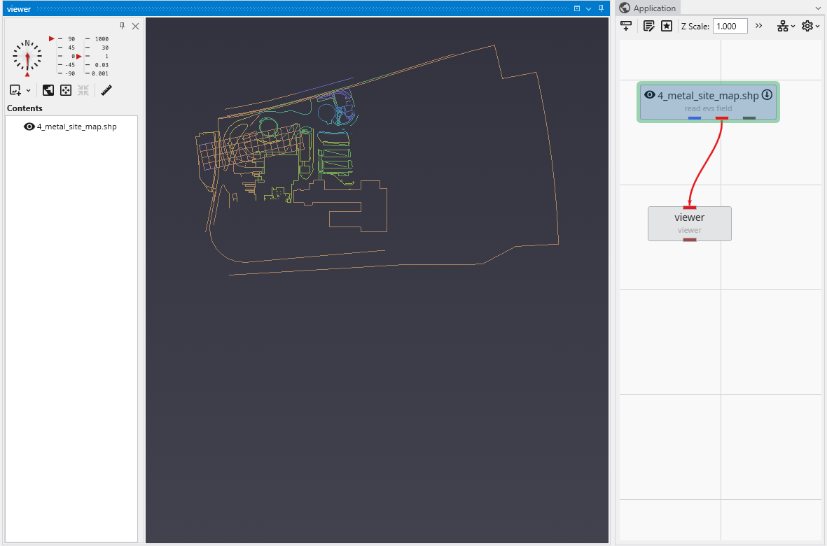
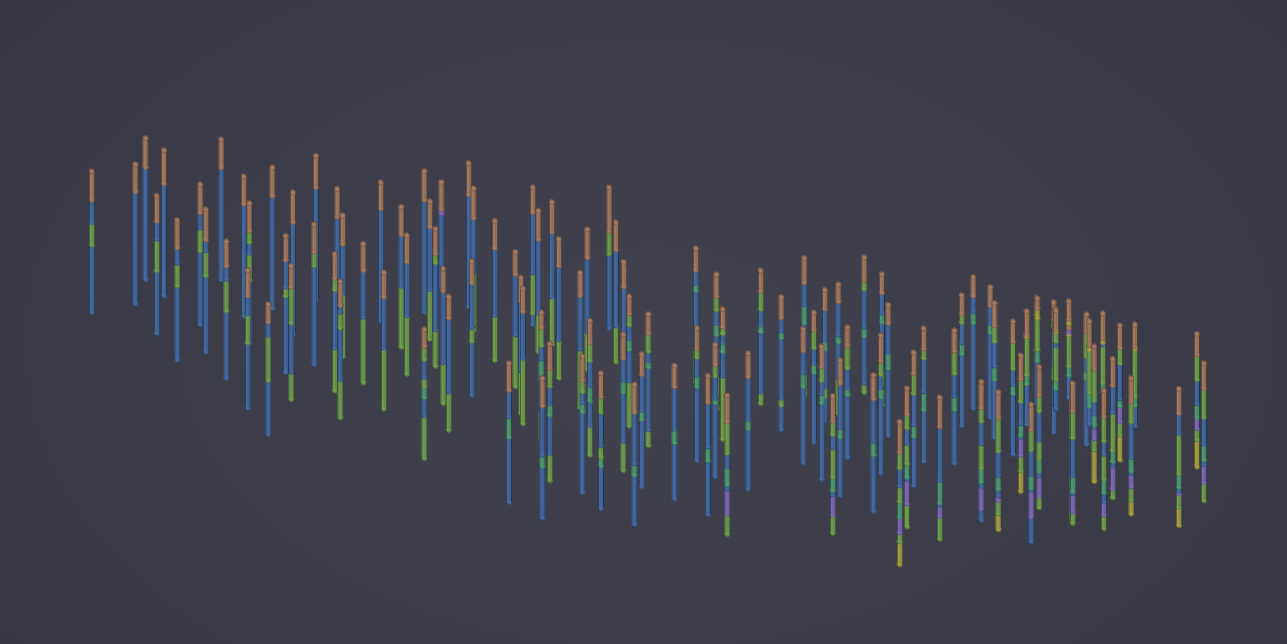
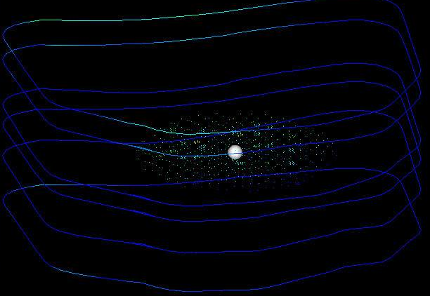
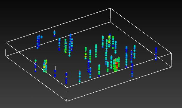
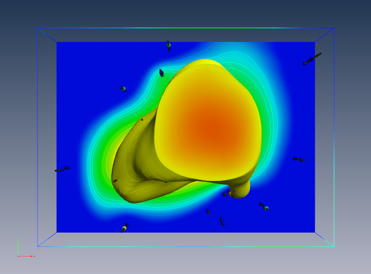
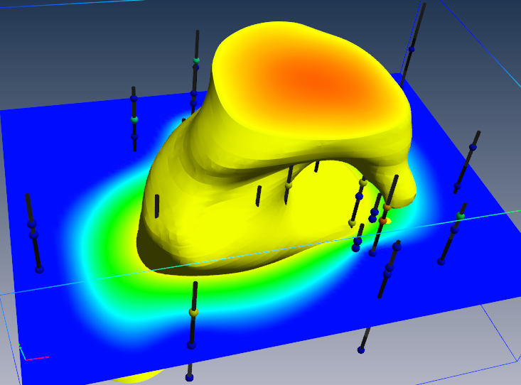
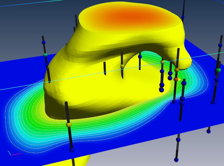
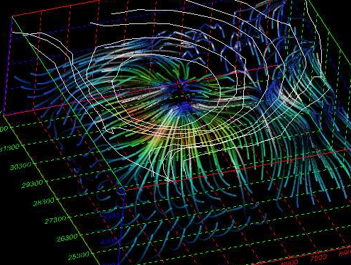
The Viewer is the primary 3D visualization window in Earth Volumetric Studio. It serves as the canvas where all the visual outputs from your Application Network - such as geologic layers, contaminant plumes, sample data, and annotations - are rendered and combined into a single, interactive scene. This is the main environment for exploring, analyzing, and presenting your 3D model.
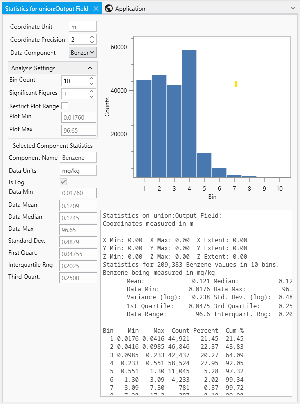
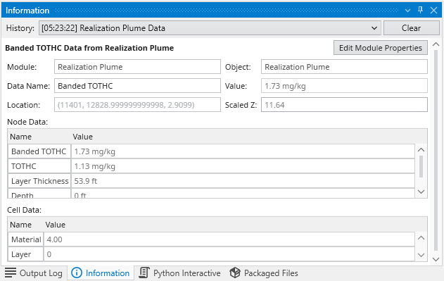
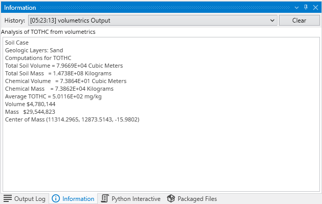
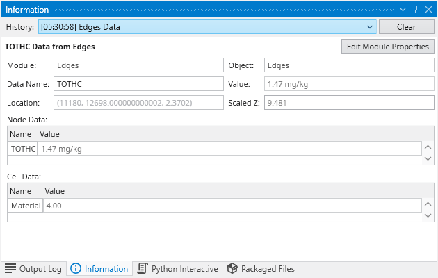
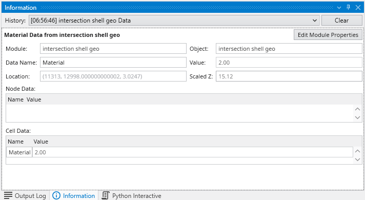
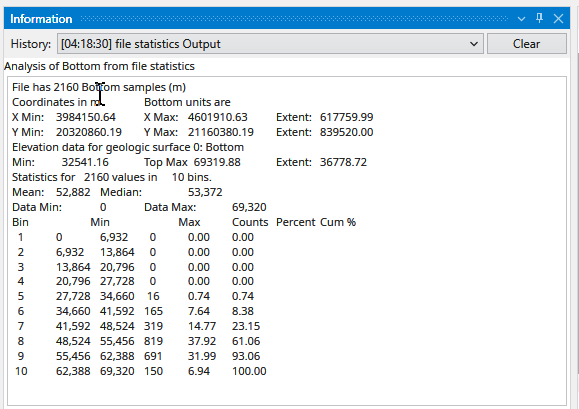
The Information Window provides detailed, contextual output from various components within Earth Volumetric Studio. Unlike the Output Log, which primarily displays text-based messages and system logs, the Information Window is designed to present data in a structured, readable, and often interactive format.
It is commonly used by modules to display analysis reports or to show detailed data about a specific point in the model that a user has “picked” in the Viewer (via Ctrl+Left Mouse Click).
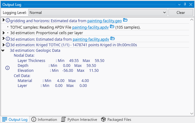
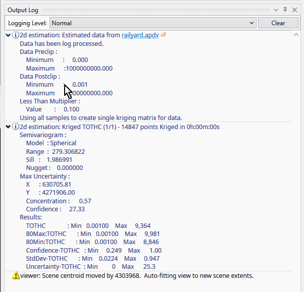
The Output Log window is a critical tool for monitoring the real-time status of Earth Volumetric Studio. It provides a chronological and hierarchical record of events, module execution details, warnings, and diagnostic messages. Whether you are running a complex analysis or troubleshooting an unexpected issue, the Output Log offers valuable insight into the application’s internal processes.
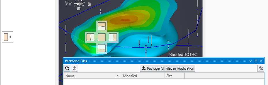
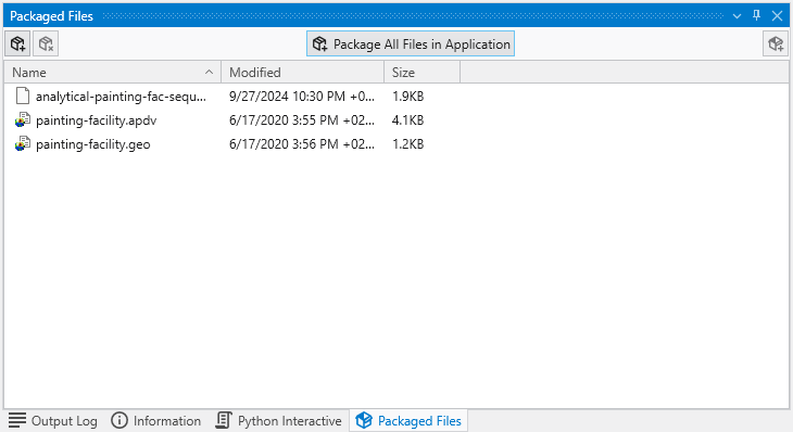
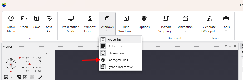
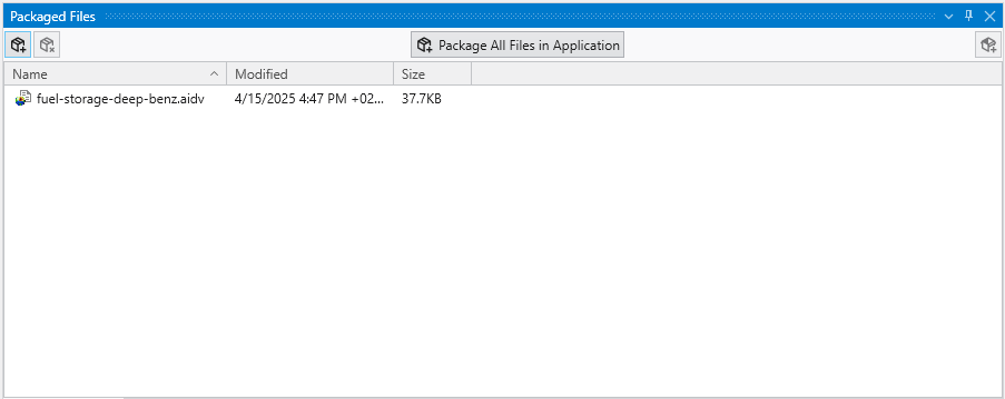
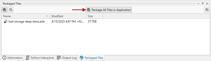
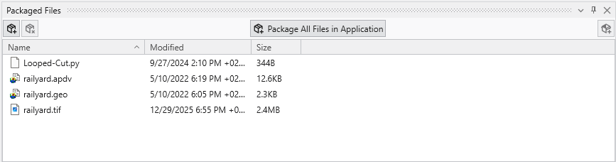
The Packaged Files feature in Earth Volumetric Studio provides a robust solution for managing project dependencies. Packaged Files are external data files that are embedded directly into your Earth Volumetric Studio application (.evs) file.
This creates a completely self-contained project, ensuring that all necessary input files are always available. It eliminates the problem of broken file paths and the need to manually copy dependent files when sharing your application with colleagues or moving it to a different computer. While this increases the size of the application file, the benefit of portability is often more important.
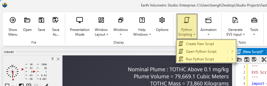
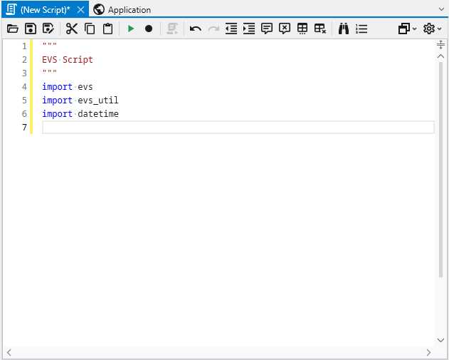
Introduction to Python Scripting Python scripting in Earth Volumetric Studio provides a method to programmatically control and automate virtually every aspect of the application. By leveraging the Python programming language, you can move beyond manual interaction to create dynamic, data-driven workflows, automate repetitive tasks, and perform custom analyses that are not possible with standard interface controls alone.
Sequences are used to create dynamic and interactive applications by managing an ordered collection of predefined “states.” A state can capture and control the properties of one or more modules simultaneously.
This functionality allows you to guide a user through a narrative or a series of analytical steps, such as changing an isosurface level, animating a cutting plane through a model, or stepping through time-based data.
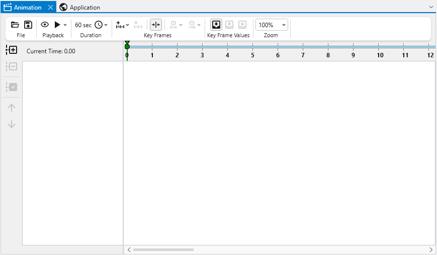
Animations in EVS Animations allow you to generate video files of smoothly changing content and views. This allows for complete control over the messaging conveyed in a single, often small deliverable file.
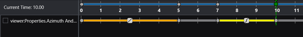
In Earth Volumetric Studio, an animation is built from one or more timelines. Each timeline represents a single, animatable property within your application. This could be anything from the camera’s position in the 3D viewer to the visibility of a specific object, a numeric value like a plume level, or the current frame of a sequence.
Subsections of The EVS Environment
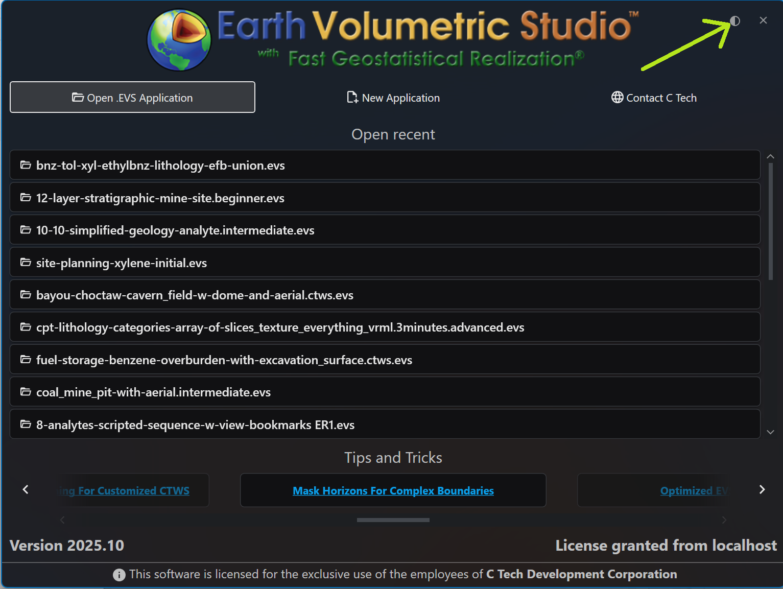
The Earth Volumetric Studio startup window is your launchpad for any project. From here, you can start with a clean slate by creating a new application, jump back into a previous project by opening an existing file, or access helpful resources.
Licensing and Version Information
The bottom of the window shows you the current version of EVS as well as well as your license status.
Alerts will also be displayed near the top of the Window when your license subscription is close to its end date. This helps with preventing an unexpected shutdown due to license subscription termination.
Navigating the Startup Screen
The startup screen provides several options to begin your session:
Open .EVS Application: Allows you to browse your file system to open any existing .evs project file.
New Application: Closes the startup screen and opens a blank workspace to begin a new project from scratch.
Open recent: Displays a list of your most recently used applications for quick access.
Additionally, the startup screen provides a button with C Tech’s contact information and links to helpful Tips and Tricks articles.
Creating a New Application
To start a project from scratch, click the New Application button.
This will immediately close the startup screen and open the main EVS workspace with a blank Application Network. This provides a clean canvas, ready for you to begin building your data processing and visualization workflow by adding and connecting modules.
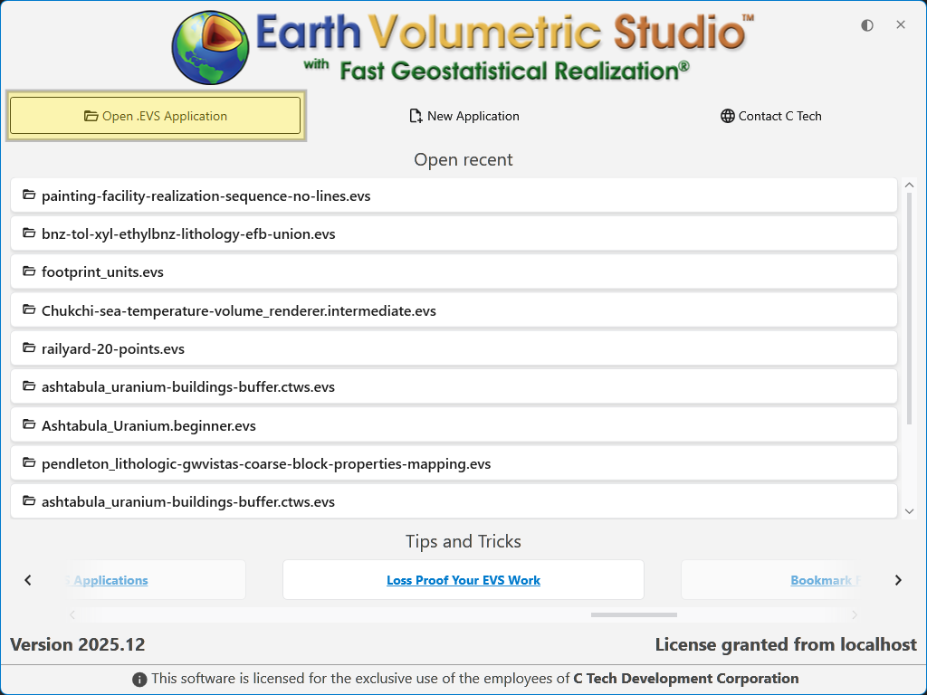
Opening an Existing Application
If you want to work on a project that is not in your “Open recent” list, you can browse your computer to find it. Click the Open .EVS Application button which will start EVS and navigate to the Open Files pane in the Menu.
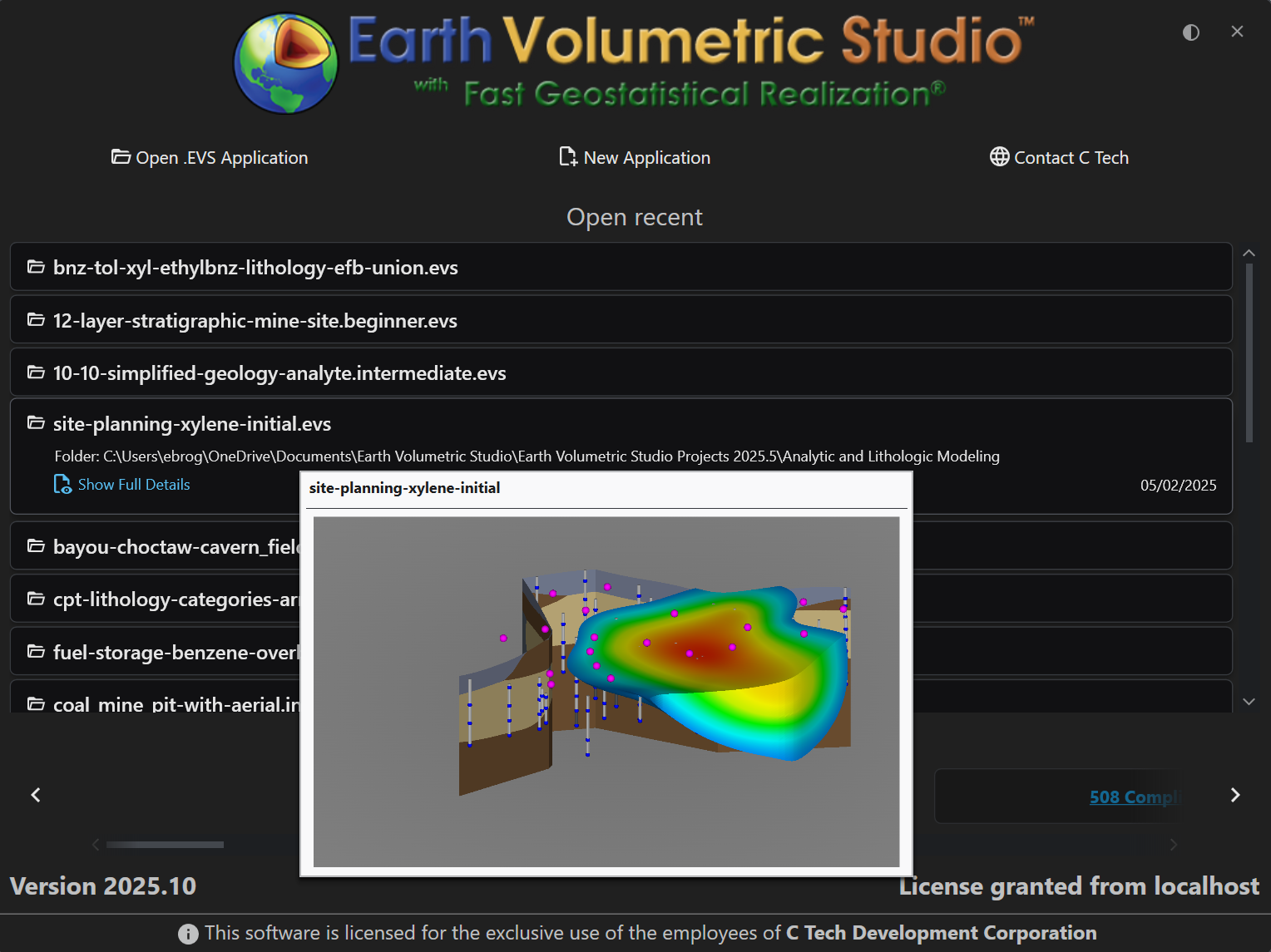
Using the Recent Applications List
The list is interactive and provides helpful information to ensure you are opening the correct project. When you hover your mouse over an application in the list, a preview window appears with key details.
Preview Window Details
The hover preview provides the following information:
Element
Description
Preview Image
A visual snapshot of the application’s 3D viewer as it appeared the last time the project was saved. This gives you an immediate visual reminder of the project’s output.
File Name
The name of the application file (e.g., site-planning-xylene-initial.evs).
Folder Path
The full directory path where the file is located on your system.
Last Modified Date
The date the file was last saved.
Show Full Details
A link that navigates to the main Open screen, where you can see more comprehensive metadata, including the application network preview.
Opening an Application
To open a project from the list, simply click directly on the application’s name. The application will load immediately, allowing you to resume your work.
Navigating to Tips and Tricks
Click on any Tips and Tricks link, which will open a browser to read the selected article.
Getting Started with the EVS User Interface
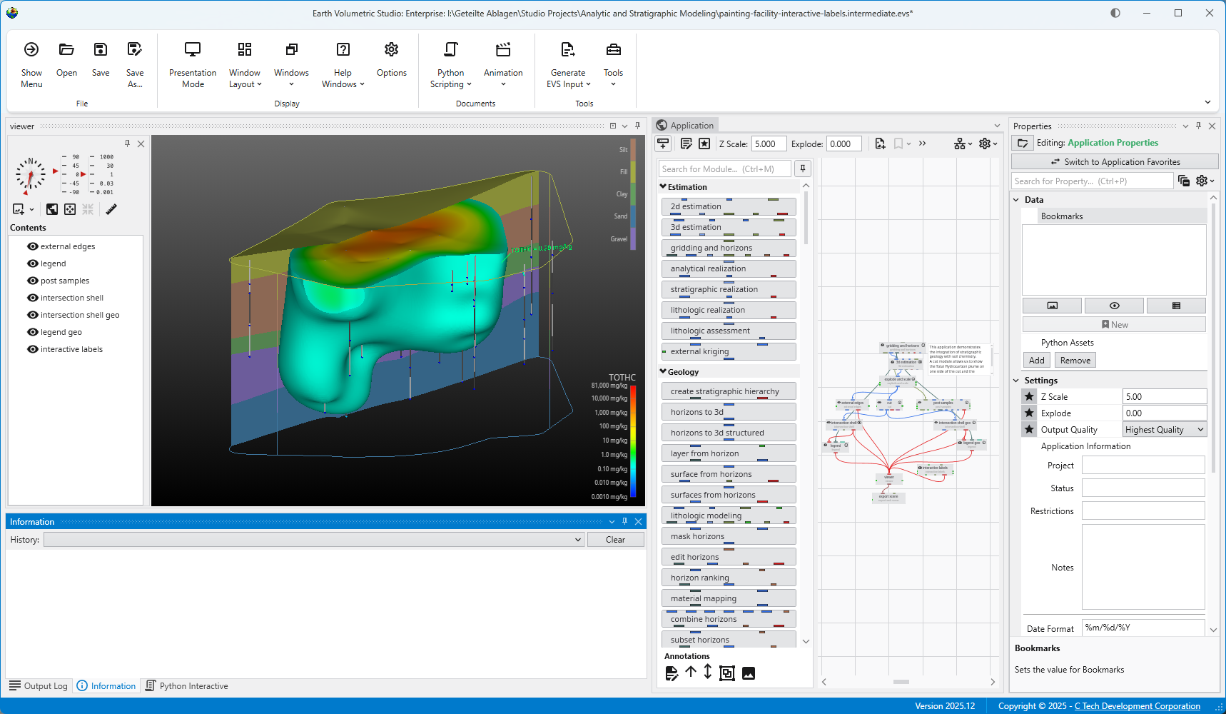
The main window is organized into five primary sections in the default layout configuration, each designed to provide a streamlined workflow for your data processing, visualization, and analysis needs. Most windows can be freely docked or undocked in any configuration and layouts can be loaded and saved.
The Main Toolbar is the row of icons at the top of the window that provides immediate access to essential commands. It is designed to help you manage your projects and control your application workflow efficiently. From here, you can perform file management tasks like opening and saving EVS applications. You can also control visual aspects of the UI by loading layouts and hiding or showing individual windows. The toolbar also includes access to automatisation through Python scripting or animations and several input file creation options.
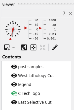
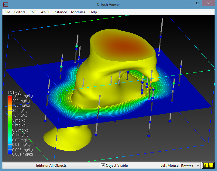
The Viewer is your primary window for 3D visualization, displaying the output of your data processing networks. It offers a suite of tools for interacting with your model. You can intuitively rotate, pan, and zoom to inspect your model from any angle. The Viewer provides dedicated controls to switch between standard viewing angles or to set a precise camera azimuth and inclination. A scene tree allows you to toggle the visibility of individual model components, helping you focus on specific parts of your data. You can also access built-in measurement tools to calculate distances directly within the 3D scene. For reports and presentations, you can capture and export the current view as high-resolution images or animations.
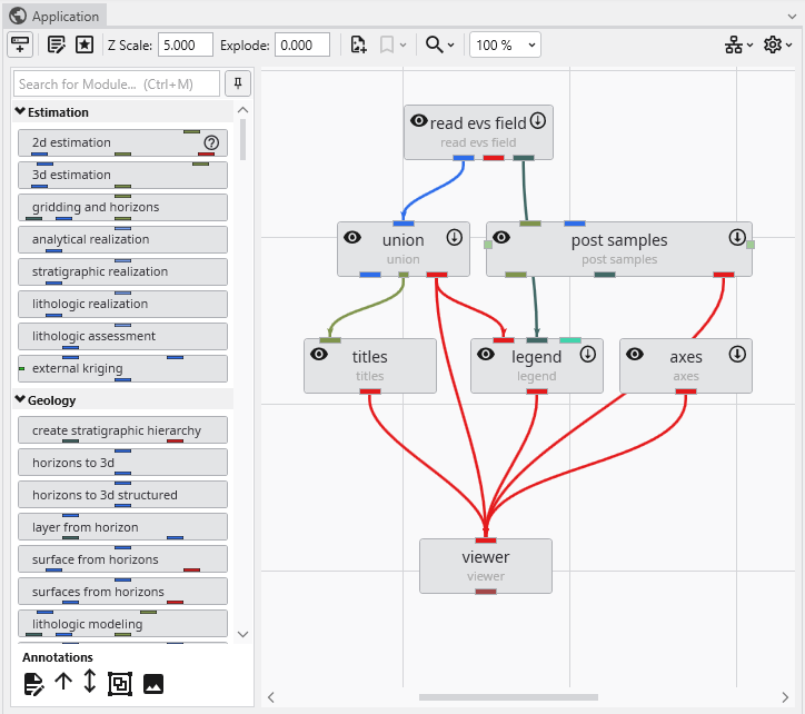
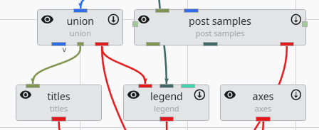
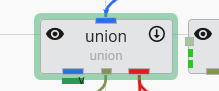
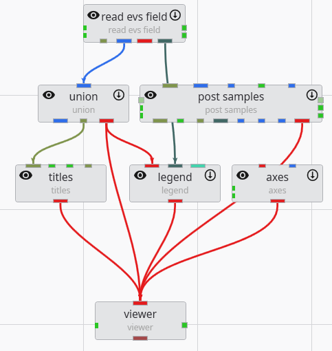
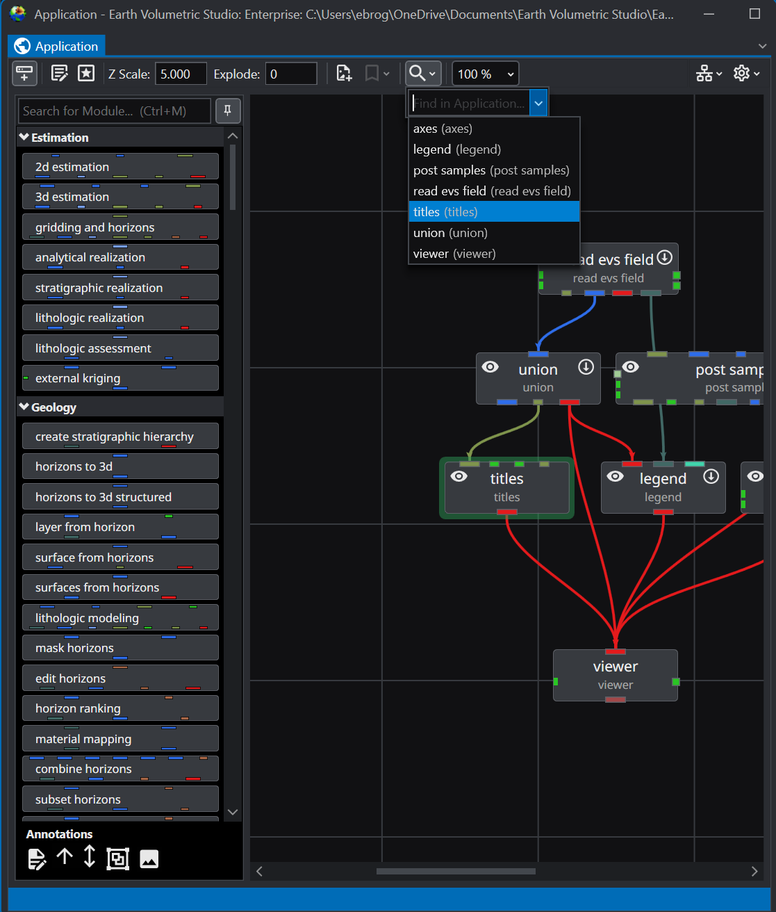
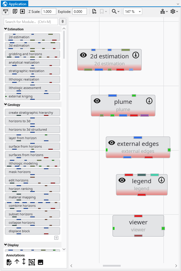
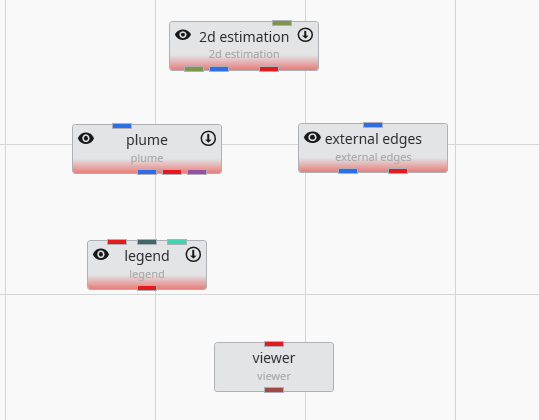
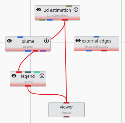
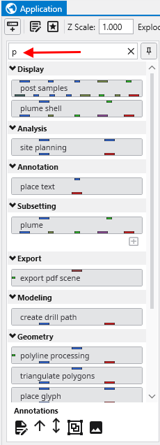
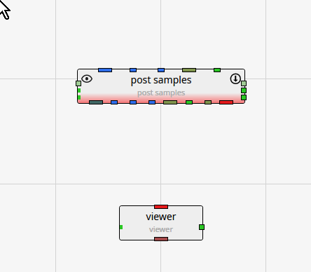
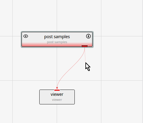
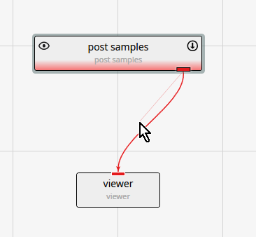
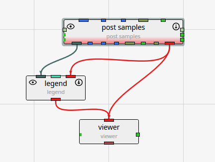
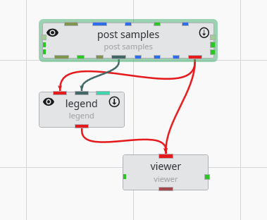
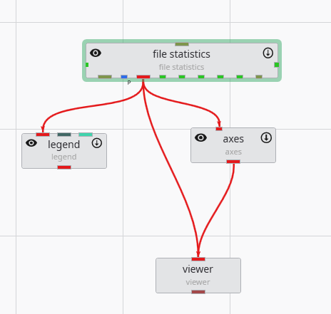
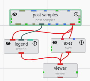
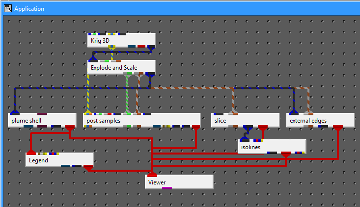
The Application Window is a dynamic, node-based workspace where you construct your data processing pipelines. This visual programming environment, often called a “pegboard,” is central to the EVS workflow. You can drag and drop modules from the module library onto this canvas, where each module represents a specific function like data input, filtering, or visualization. To create complex workflows, you draw connections between modules to define the flow of data from inputs through various processing steps to the final outputs. The connection style can be customized to use either curved or straight lines. You can also organize and group modules to create logical and readable application networks.
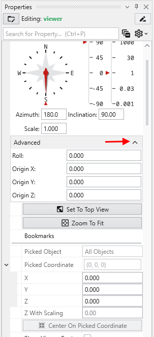
This multi-functional section allows you to configure every aspect of your project. When a module is selected in the Application Window, this panel displays all of its configurable parameters, allowing you to control how it processes data. You can also modify global settings that affect the entire project, such as adjusting the vertical exaggeration with z-scale or separating objects for better visibility with an explode factor. This area also lets you save and manage specific camera positions as bookmarks, enabling you to quickly return to important views. The Application Favorites allows you to build a custom collection of frequently used or important module and application properties.
5. Output Log, Information, and Python Interactive Panel
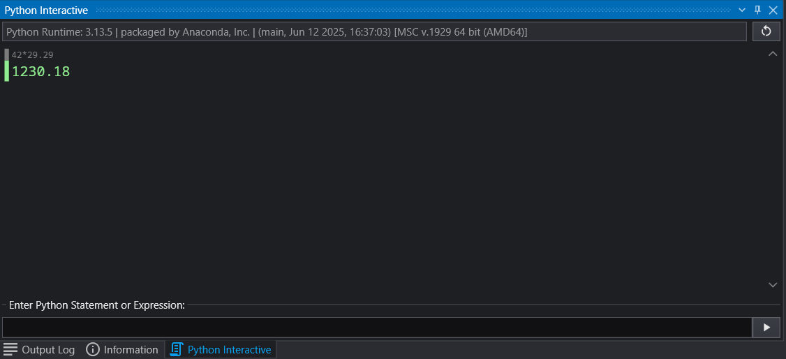
This tabbed panel at the bottom of the screen provides critical feedback, logs, and advanced scripting capabilities. The Output Log displays the information your modules provide, along with execution warnings and errors. The Information tab provides details about probed locations or objects and the data at the probe point. For advanced users, the integrated Python Interactive Panel offers a full scripting console to programmatically control the EVS application, manipulate data, and extend the built-in functionality.
The application’s user interface is highly customizable, allowing you to arrange tool windows like the Viewer, Properties, and Application Network to best suit your workflow. Windows can be “docked” to the edges of the main application or other window, grouped with other windows in tabs, or “floated” as independent windows on your desktop. This flexibility enables you to create a personalized layout that keeps the tools you need most frequently within easy reach.
Subsections of Main EVS Window
The application’s user interface is highly customizable, allowing you to arrange tool windows like the Viewer, Properties, and Application Network to best suit your workflow. Windows can be “docked” to the edges of the main application or other window, grouped with other windows in tabs, or “floated” as independent windows on your desktop. This flexibility enables you to create a personalized layout that keeps the tools you need most frequently within easy reach.
Window Title Bar and Context Menu
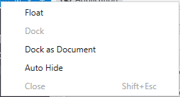
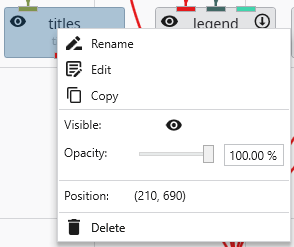
Each tool window has a title bar containing several controls for managing its state. You can access these functions by right-clicking the title bar or by using buttons provided on the title bar directly.
Undocking and Floating Windows
A floating window is one that is detached from the main application window and can be moved freely around your screen, even to a second monitor. To make a window float:
Drag the Title Bar: Click and hold the title bar of any docked window and drag it away from the edge. As you drag it towards the center of the screen, it will detach and become a floating window.
Drag the Tab: For windows docked as tabs in same pane as other windows, drag the window by its tab.
Use the Context Menu: Open the window’s context menu and select the Float option. The window will immediately detach from its docked position.
Docking Windows
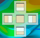
To dock a floating window, simply drag it by its title bar. As you move it over the main application window or any floating window, a set of docking guide icons will appear. Dropping the window onto one of these icons will dock it to the corresponding location.
Edge Docking: The four arrow icons at the edges of the screen will dock the window to the top, bottom, left, or right side of the main application, spanning its full width or height.
Pane Docking: The five-icon control that appears in the center of an existing window pane allows for more precise placement. The four outer arrows will dock the window to the side of that specific pane, creating a split view. The center icon will dock the window as a new tab within that pane group.
Document Area: One pane is designated as the central document area. It occupies the main, central space of the application window. The other docking guides for top, bottom, left, and right positions are usually arranged around this central area.
Context Menu Docking: You can also use the context menu of a floating window. Dock will typically return it to its last docked position, while Dock as Document will place it as a tab in the central document area.
Note: The Application window is the central point of any EVS application and layout. It can only be either docked in the Document Area or made a floating window.
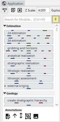
Auto-Hiding Windows (Pinning)
The Auto-Hide feature allows you to keep windows accessible without them permanently taking up screen space. You can control this using the pin icon in the window’s title bar or the Auto Hide option in the context menu.
Pinned (Vertical Pin): When the pin icon is vertical, the window is pinned open. It will remain visible in its docked location.
Unpinned / Auto-Hidden (Horizontal Pin): When the pin icon is horizontal, the window is set to auto-hide. It will collapse into a named tab on the edge of the window. To temporarily view it, simply hover your cursor over its tab. It will slide out for you to use and slide away again when you move your cursor off it. To keep it open, click the pin icon to return it to the pinned state.
Saving and Loading Layouts
When you created a layout you like, you can save it through the Options in the Menu. Layouts can be switched to previously saved ones through either the Menu or the Window Layouts button in the Main Toolbar.
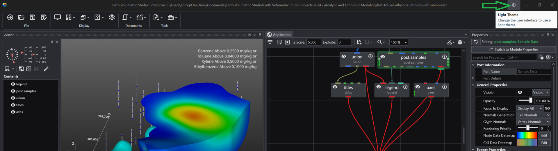
The application offers both a Light and a Dark theme to customize the appearance of the user interface. This choice is purely a matter of personal preference and does not affect the application’s functionality or the output of your visualizations. You can switch between themes at any time to best suit your working environment and visual comfort.
Choosing Your Theme: Light vs. Dark
Selecting a theme can have a significant impact on readability and eye comfort depending on your work environment and personal preferences.
Dark Theme: The dark theme uses a dark background with light-colored text. Many users find this reduces eye strain, especially when working for long periods or in low-light conditions. It can also help reduce screen glare and improve focus on the central content by making the surrounding interface elements recede.
Light Theme: The light theme provides a traditional light background with dark text. This often offers superior readability in brightly lit environments, such as a well-lit office or a room with significant natural light. For some users, the high contrast of dark text on a light background can appear sharper and more familiar.
How to Change Themes
You can switch between the Light and Dark themes from three different locations within the application.
1. Setting the Default Theme in Options
To set your preferred theme that the application will use every time it starts, you can use the Options window.
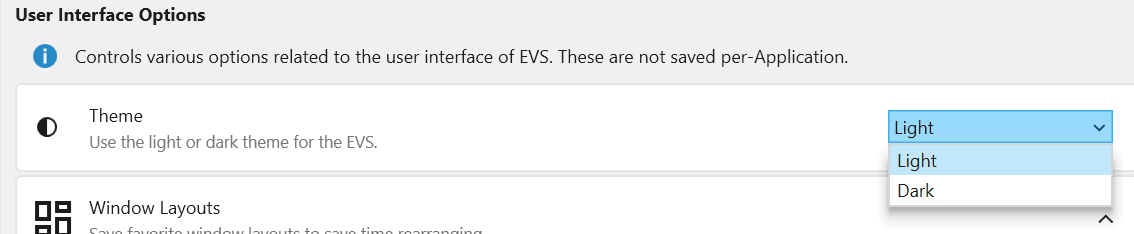
Navigate to the main application Menu > Options.
In the Options window, select User Interface Options.
Under “Color Options for Applications”, choose your desired theme.
2. Toggling on the Launch Window
When you first start the application, you can quickly toggle the theme directly from the launch window before opening a project. Click the half-moon icon in the upper-right corner to switch between the Light and Dark themes.
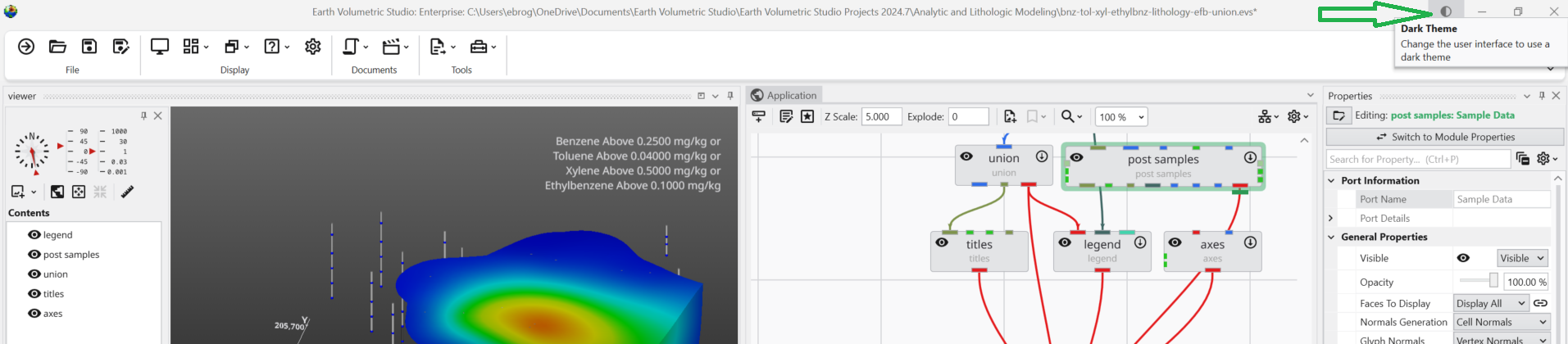
3. Toggling in the Main Application Window
You can also switch themes on-the-fly while you are working. In the upper-right corner of the main application window, you will find the same half-moon icon. Clicking this icon will instantly toggle the interface between the Light and Dark themes, allowing you to adapt to changing lighting conditions or preferences without interrupting your workflow.
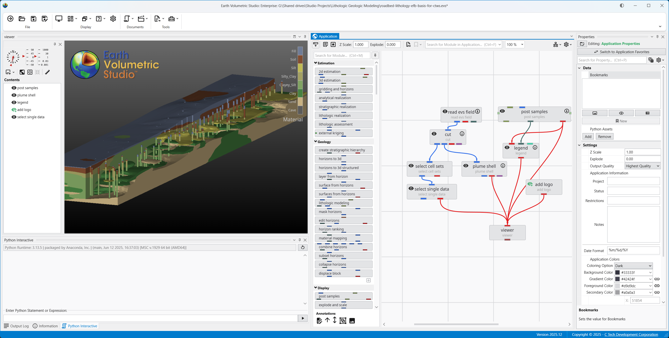
Main window with Light Theme active:
Main window after toggling to Dark Theme:
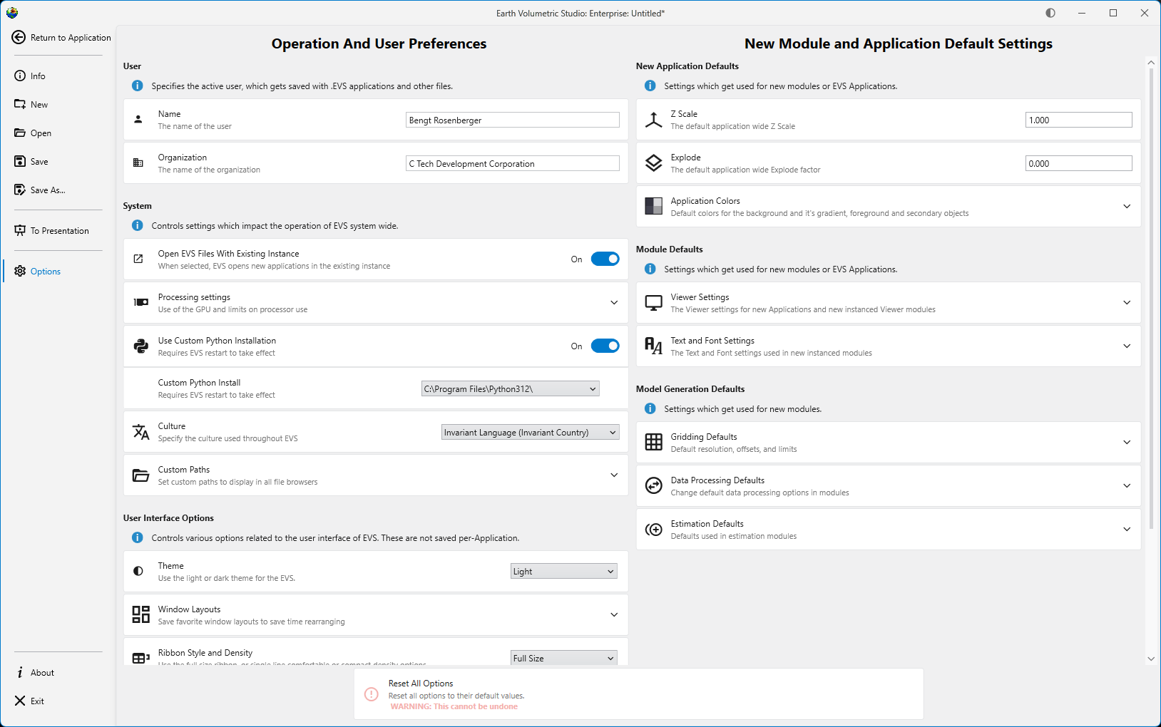
The Main Toolbar
The Main Toolbar is the primary command bar in Earth Volumetric Studio, located at the top of the main application window. It provides streamlined access to the application’s most common features and functions. The toolbar is organized into logical sections: File, Display, Documents, and Tools, making it easier to locate and use the necessary commands for your projects.
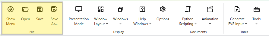
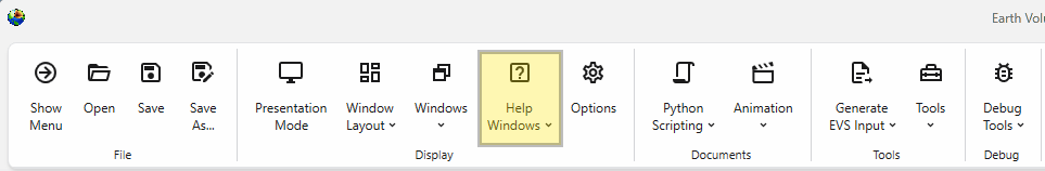
File
This section contains essential commands for file management.
Button
Description
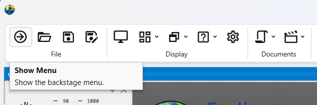
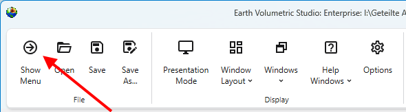
Show Menu
Opens the main application menu, which provides access to a comprehensive list of commands, including those not present on the Main Toolbar.
Open
Provides quick access to open Earth Volumetric Studio project files.
Save
Saves the currently active project. If the project has not been saved before, it will prompt you for a file name and location.
Save As…
Saves the current project under a new name or in a different location.
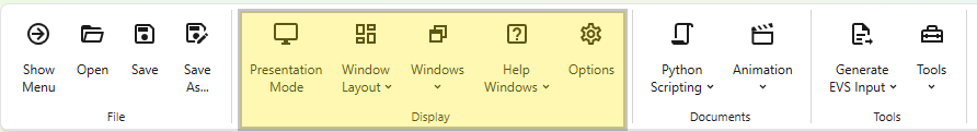
Display
This section provides tools to manage the application’s user interface, windows, and general options.
Toggles a full-screen mode that maximizes the viewer and hides certain UI elements, ideal for presentations.
Window Layout
A dropdown menu that allows you to quickly load saved window layout configurations. Use the Windows Layouts section in the Options menu to create new layouts.
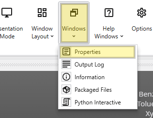
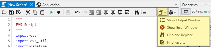
Windows
A dropdown menu to show, hide, or bring focus to specific windows within the application, such as the Properties or Output Log windows.
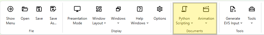
A dropdown menu that provides access to the Python scripting interface, allowing you to create, open, and run Python scripts to automate tasks and extend functionality.
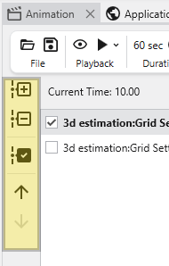
A dropdown menu for creating and opening animations. This includes commands for the Animation Control panel, which allows you to define keyframes and playback your animated sequences.
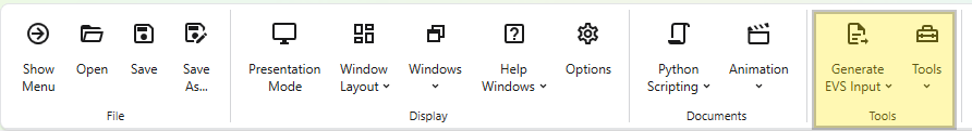
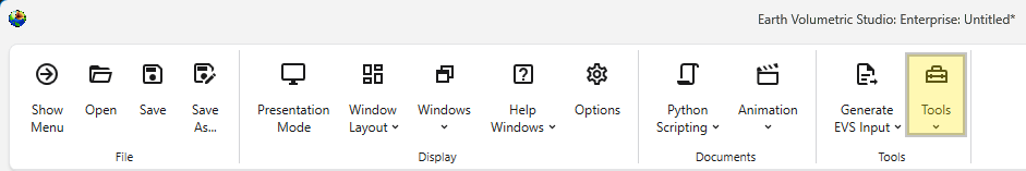
Tools
This section contains a collection of specialized tools and utilities.
A dropdown menu that provides access to a variety of supplementary tools and utilities available within the application.
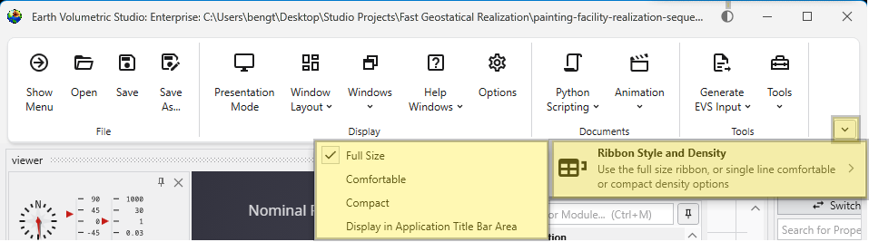
Toolbar Styles
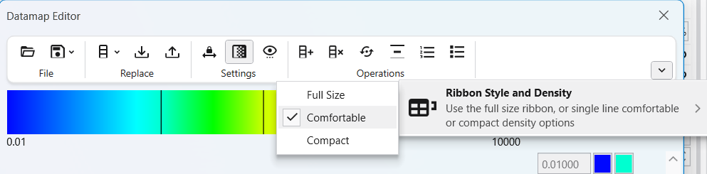
You can customize the appearance of the Main Toolbar to suit your preferences. Right-click anywhere on the toolbar to open the “Ribbon Style and Density” menu, or use the arrow to the right of the toolbar.
These settings can also be configured in the main Options dialog in the Menu. The available styles are detailed below.
Style
Description
Example
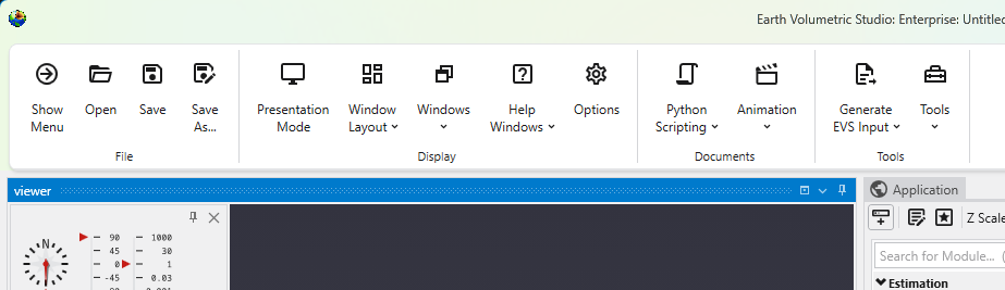
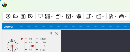
Full Size
The default style, featuring large buttons with descriptive text for clarity.
Comfortable
A more compact style that reduces the size of buttons and text, providing a balance between usability and screen space.
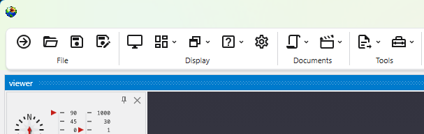
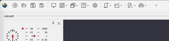
Compact
The most space-efficient style, displaying only icons without text labels for a minimal footprint.
Display in Application Title Bar Area
This option moves the toolbar into the application’s title bar, freeing up additional vertical space in the main window.
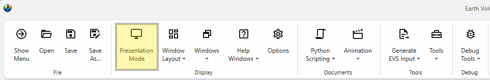
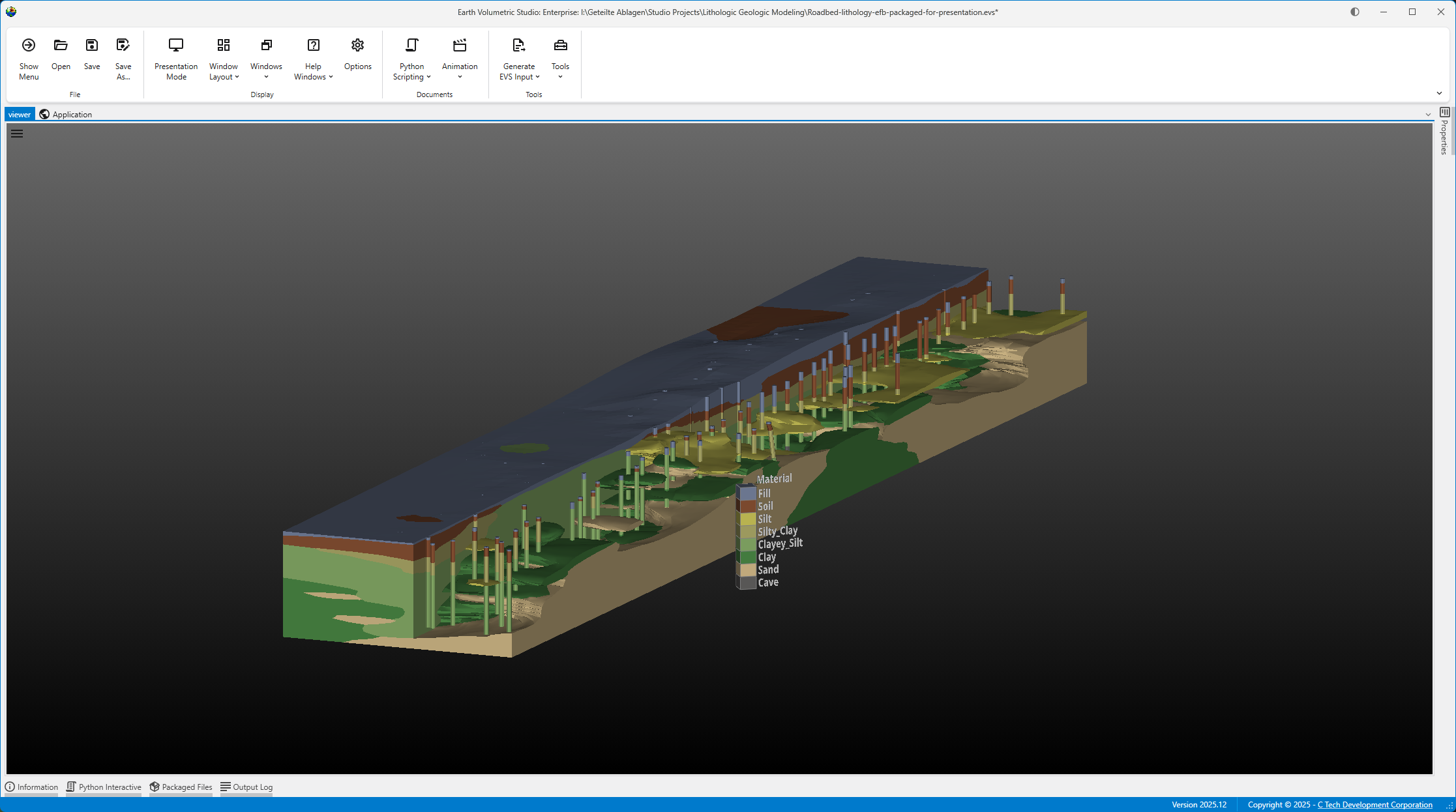
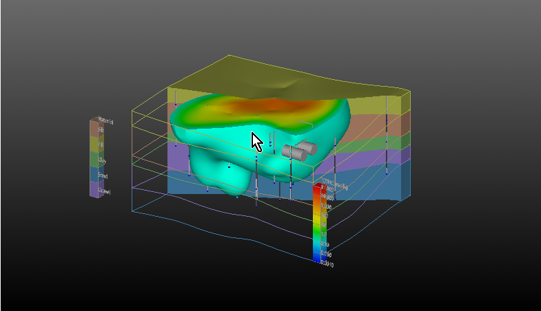
Presentation Mode optimizes the user interface for interacting with a completed application. It simplifies the workspace by hiding development-focused UI elements, allowing you to focus on the application’s controls and outputs.
Accessing Presentation Mode You can enable Presentation Mode using the Presentation Mode button in the Main Toolbar.
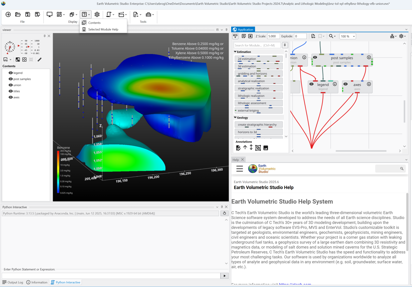
Accessing Help The help can be found through the Help Windows button in the Main Toolbar.
General Application Help For general information, searching, and browsing all help topics, you can use the main Help window.
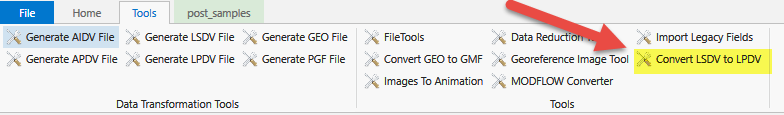
The Tools menu provides a collection of utilities for file conversion, data processing, and creating animations. These tools are designed to help you prepare your data for use in EVS.
Accessing Tools The Tools button can be found in the Main Toolbar. Clicking it will open a list of available tools.
Subsections of Main Toolbar
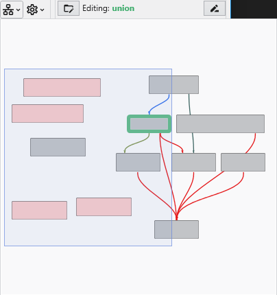
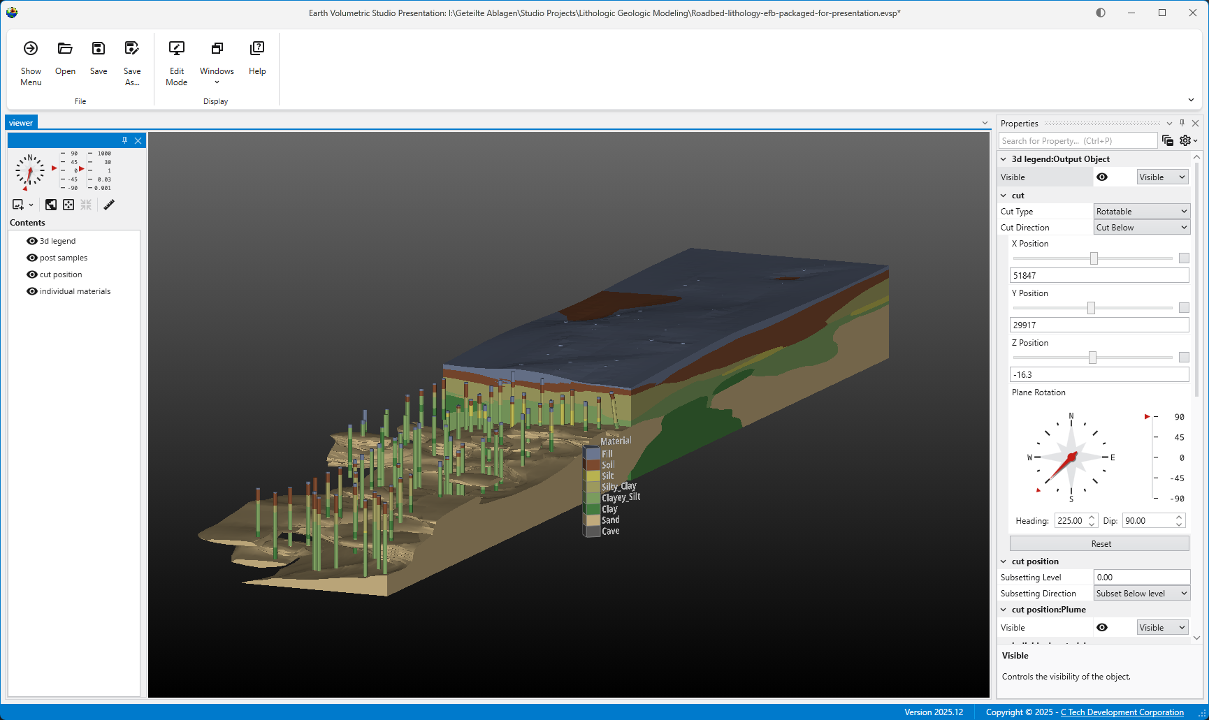
Presentation Mode optimizes the user interface for interacting with a completed application. It simplifies the workspace by hiding development-focused UI elements, allowing you to focus on the application’s controls and outputs.
Accessing Presentation Mode
You can enable Presentation Mode using the Presentation Mode button in the Main Toolbar.
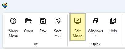
Presentation mode can be left using the Edit Mode button in the Main Toolbar. This button is only visible when Presentation Mode is active.
Purpose of Presentation Mode
Presentation Mode provides a cleaner, more streamlines experience ideal for presenting your work or for any scenario where you are primarily executing and interacting with the application rather than building or modifying it.
For this reason, the following elements are hidden or inactive:
Application Window: The window containing the application workflow and for adding new modules is hidden.
Module and Port Connections: The ability to create or modify connections between modules is disabled.
Main Toolbar: Most buttons focused on creating applications are hidden.
Presentation Mode vs. EVS Presentation Files
While Presentation Mode is similar to the view when loading an EVS Presentation file, it is less restrictive. An EVS Presentation file (.evsp) is a self-contained, read-only version of an application that limits user editing and intended for delivery to end users. Its main purpose is for distribution to clients who need to run an application and change predetermined properties, but not modify it.
In contrast, Presentation Mode still allows for editing of module and application properties and options. It is merely a simplified user interface. This provides a flexible way to display interactive applications that are simplified for presentations but not entirely locked down.
This action opens the main Help window, where you can search for topics.
Module-Specific Help
When the Module Help window is opened, any module being edited (selected in the application window) will also show its help contents in the Module Help window. As you edit different modules, the Module Help will reflect the currently selected module.
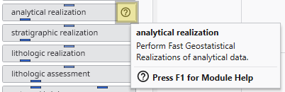
To get help for a module which hasn’t been instanced, follow these steps:
Hover your mouse over the question mark in the desired module in the Module Library.
Wait for the module’s tooltip to appear:
While the tooltip is visible, press the F1 key.
This will open the Module Help window containing specific information for that module.
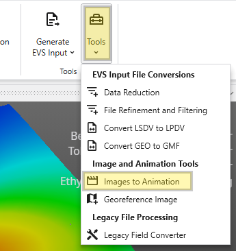
The Tools menu provides a collection of utilities for file conversion, data processing, and creating animations. These tools are designed to help you prepare your data for use in EVS.
Accessing Tools
The Tools button can be found in the Main Toolbar. Clicking it will open a list of available tools.
Tool Buttons
EVS Input File Conversions
This section contains tools for processing and converting various data files into formats optimized for EVS.
Tool
Description
Data Reduction
This utility helps you manage large datasets by reducing the number of data points. It can be used to sample or filter your data, which can improve application performance and reduce processing times with configurable loss of detail. It is used to get optimal results when kriging dense data. See the Dense Data tutorial video.
File Refinement and Filtering
Use this tool to clean and refine your data files. It allows you to apply filters to remove outliers, correct errors, or extract a specific subset of your data based on defined criteria, ensuring higher quality input for your models.
This tool converts the Borehole Geology(.geo) file format into the Geology Multi-File (.gmf) format. This is useful if you want to replace a single surface in a GEO hierarchy (such as the ground surface) with more high-resolution data that is not synchronous with your .GEO borings.
Image and Animation Tools
This group of tools helps you create animations and prepare images for use in your projects.
Tool
Description
Images to Animation
This utility takes a sequence of individual image files and compiles them into a single animation video. This is useful for creating time-lapse visualizations of your models or other dynamic presentations.
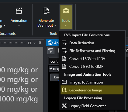
Georeference Image
Creates and edits world files or .gcp (ground control point) files for images. Use this tool to assign real-world geographic coordinates to a raster image, such as an aerial photograph or a scanned map. Georeferencing allows the image to be accurately positioned and scaled within your 3D scene alongside other spatial data.
Legacy File Processing
This section provides tools for working with older, outdated file formats.
Tool
Description
Legacy Field Converter
Reads older format files that can contain EVS Fields, such as Field (.FLD), UCD (.INP) and netCDF files (.CDF) and converts them to standard EVS Field File format (.EFB). The .EFB format is used because it is the smallest and old file formats do not require the more complex features that the .EF2 format allows.
The Images To Animation tool allows you to compile a sequence of individual image files into a single video animation. This is ideal for creating time-lapse visualizations, showcasing model changes over time, or presenting a series of related images, for example written by EVS through sequences and Python Scripting, as a dynamic video.
The Georeference Image tool is a useful utility for assigning real-world geographic coordinates to raster images. This process, known as georeferencing, allows you to accurately overlay images with other spatial data in your project. The tool enables you to create and edit world files (e.g., .jgw, .tfw) or ground control point files (.gcp), which store the image’s location, scale, and orientation information.
Subsections of Tools
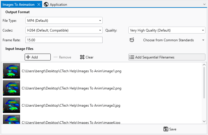
The Images To Animation tool allows you to compile a sequence of individual image files into a single video animation. This is ideal for creating time-lapse visualizations, showcasing model changes over time, or presenting a series of related images, for example written by EVS through sequences and Python Scripting, as a dynamic video.
Before creating your animation, you can configure the output settings to meet your specific needs for quality, file size, and compatibility.
Setting
Description
Frame Rate
Determines the number of frames (images) displayed per second. You can enter a custom value or select from standard presets:
60 FPS
30 FPS
NTSC (29.97 FPS)
PAL (25 FPS)
File Type
Lets you choose the container format for your output video file.
MP4 (Default): A widely supported modern option with a good balance of quality and file size.
AVI: An older, less compressed option that may result in larger files.
WebM: An open-source choice designed for web use, providing efficient compression.
Quality
Controls the trade-off between visual quality and file size.
Lossless: Preserves the exact quality of the source images but results in very large files.
Very High & High Quality: Produce excellent quality with efficient compression.
Medium & Low Quality: Offer progressively more compression for smaller file sizes, with some loss of visual detail.
Codec
Determines the compression algorithm used to encode your video.
H264: A highly compatible codec supported by most devices and platforms.
H265: A newer codec offering better compression than H264, resulting in smaller file sizes for the same quality.
H264RGB: A variant of H264 that preserves full color information, ideal for technical or scientific visualizations.
Managing Files
The File List section is where you add and manage the images that will make up your animation.
Function
Description
The File List View
This area displays the list of images you have added. Each entry shows a small preview thumbnail of the image on the left and its full file path on the right. The order of the files in this list determines the sequence in which they will appear in the final animation.
Adding and Removing Files
To add images, click the Add button to open a file dialog, where you can browse for and select one or more files. To remove a specific image, select it from the list and click the Delete button. The Clear button will remove all images from the list, allowing you to start over.
Adding Sequential Filenames
When the Add Sequential Filenames toggle is enabled, the behavior of the Add button is modified to streamline the import of numbered image sequences. If you select a single file that has a number at the end of its name (e.g., image1.png), the tool will automatically search for and add all other files in the same directory that share the same base name and have a matching extension (e.g., image2.png, image3.png, etc.).
Note that this feature requires both the file extension and the base filename (the part before the number) to match exactly. For example: Adding image1.png would add image2.png, but not image3.jpg because of its differing extension. |
About source image sizes
You may encounter a warning messages about image dimensions during conversion. This occurs because most video codecs require the dimensions of the video frame (both width and height) to be even numbers. This requirement is due to the way video compression algorithms process images. If a source image has an odd dimension, the encoder may not be able to process it. To ensure compatibility, the Images to Animation tool will automatically resize the image to the nearest even resolution before adding it to the video. While this automatic resizing is necessary for the video encoding process, it may result in a slight loss of image quality or the softening of fine features in the image.
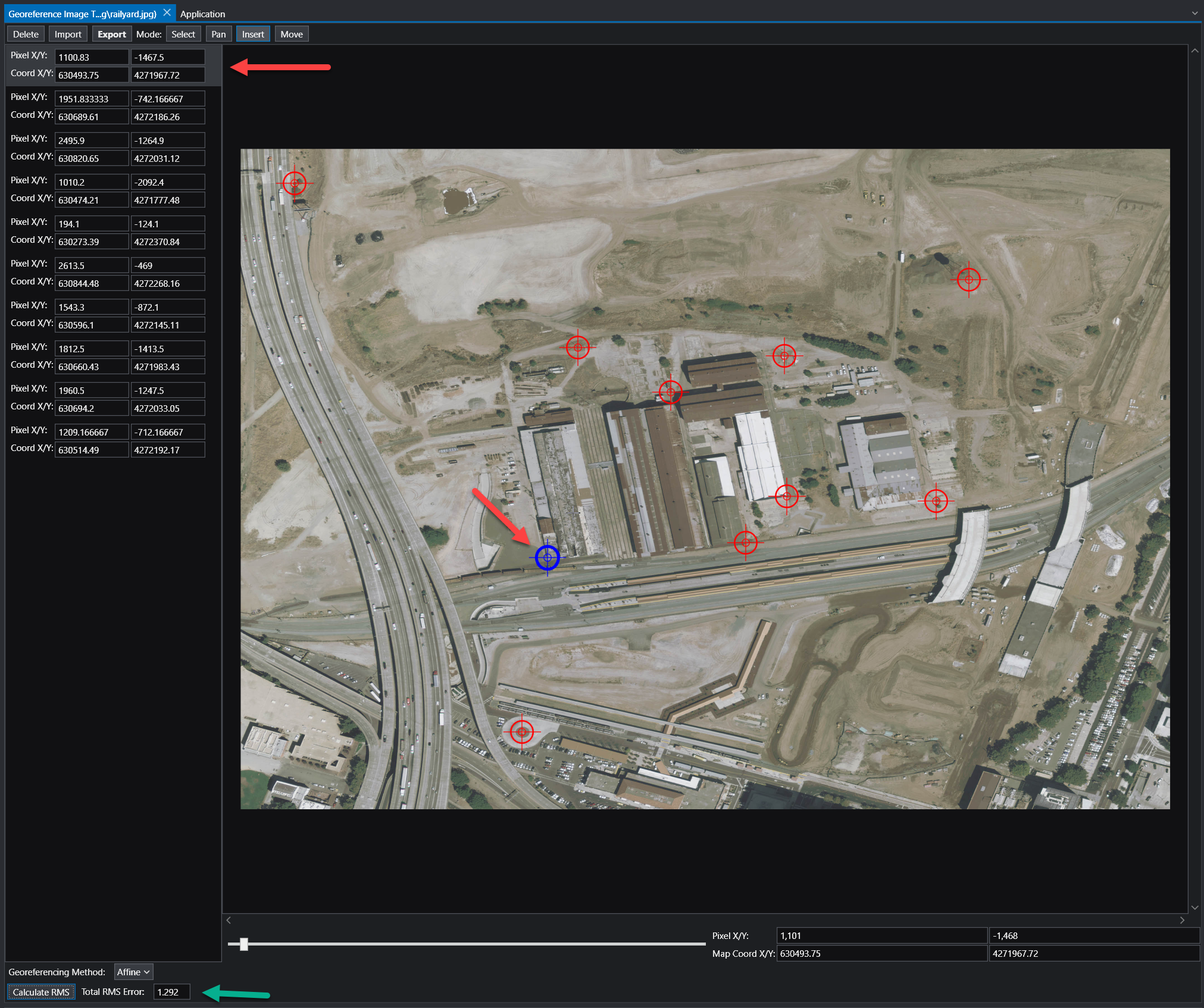
The Georeference Image tool is a useful utility for assigning real-world geographic coordinates to raster images. This process, known as georeferencing, allows you to accurately overlay images with other spatial data in your project. The tool enables you to create and edit world files (e.g., .jgw, .tfw) or ground control point files (.gcp), which store the image’s location, scale, and orientation information.
When you launch the tool, you will first be prompted to open an image file. Once loaded, the main interface provides all the necessary functions to link pixel coordinates on the image to known map coordinates.
Accessing the Georeference Image tool
The Georeference Image tool can be opened from the main Tools tab in the Main Toolbar.
Interface Overview
The Georeference Image tool is organized into several key areas:
Component
Description
Image Panel
The central part of the window displays your image. This is your primary workspace for viewing the image and placing, selecting, and moving ground control points.
GCP List
The panel on the left lists all the Ground Control Points (GCPs) for the current image. Each point has an entry showing its pixel coordinates (Pixel X/Y) and the corresponding map coordinates (Coord X/Y).
Toolbar
Located at the top, the toolbar provides access to the main functions for managing GCPs and the georeferencing process.
Status Bar
The area at the bottom of the window displays important information, including the georeferencing method, accuracy metrics, and live coordinate readouts for your cursor’s position.
Workflow: How to Georeference an Image
Georeferencing involves creating links between points on the image and their known real-world coordinates. These links are called Ground Control Points (GCPs).
Choose a Georeferencing Method:
Use the Georeferencing Method dropdown in the status bar to select the mathematical model that will be used to transform the image from pixel coordinates to map coordinates. The best method depends on the quality of the image and the number of GCPs you have. The available methods are:
Map to Min/Max: Stretches the image to fit a bounding box defined by two GCPs representing the minimum and maximum map coordinates. Requires 2 GCPs.
Translate: Shifts the entire image based on the location of a single GCP without any rotation or scaling. Requires 1 GCP.
2 Point Translate / Rotate: Moves and rotates the image to align with two GCPs, but does not perform any scaling. Requires 2 GCPs.
Translate / Scale: Moves and uniformly resizes the image to fit two GCPs, but does not perform any rotation. Requires 2 GCPs.
Affine: A first-order polynomial transformation that can perform translation, scaling, rotation, and skewing. This is a versatile and common method for standard georeferencing. Requires a minimum of 3 GCPs. This is the recommended option, but requires at least 3 GCP points to be specified.
2nd, 3rd, and 4th Order: These are higher-order polynomial transformations used to correct for more complex, non-linear distortions in an image (e.g., lens distortion or terrain relief). They require progressively more GCPs (a 2nd Order transformation needs at least 6 GCPs) and should be used when a simpler model like Affine is not sufficient.
Add Ground Control Points:
Set the Mode on the toolbar to Insert.
Zoom and pan to a recognizable feature on the image (e.g., a road intersection, a building corner).
Click on the feature. A new entry will be created in the GCP in the list on the left of the pixel location selected.
Alter the X/Y coordinates to your desired real-world coordinates.
Repeat this process for several points distributed across the image.
Review Accuracy:
Once you have enough GCPs for your chosen method, click the Calculate RMS button. The Total RMS Error value will update. This value represents the root mean squared error, which is a measure of the average distance between the true map locations of your GCPs and their calculated locations based on the current transformation. A lower RMS error indicates a more accurate fit.
Export the Georeference File:
When you are satisfied with the accuracy, click the Export button on the toolbar. This will save the coordinate information to a file (e.g., a world file or a .gcp file) that accompanies your image.
NOTE: In general, add as many control points as possible. More control points will almost always result in a better georeferencing, as any error due to precision will be averaged out across all of the entered control points. Our recommendation is to use an Affine transformation method (which is typically the industry standard) with as many control points as possible. While three is the minimum required, ten or more is typically recommended.
Toolbar Functions
Function
Description
Delete
Deletes the currently selected GCP.
Import
Loads GCPs from an existing file (e.g., a .gcp file).
Export
Saves the current set of GCPs to a world file or .gcp file. The .gcp files are compatible with ArcGIS image link files.
Mode
Select: Allows you to select a GCP from the list or by clicking it on the image.
Pan: Allows you to pan around the image by clicking and dragging. You can also pan using the middle mouse button.
Insert: Enables you to add new GCPs by clicking on the image.
Move
Allows you to adjust the position of a selected GCP. After clicking this button, select a GCP and click its new desired location on the image to update its pixel coordinates.
Interpreting Coordinates
Once an image is georeferenced, you can use the tool to find the map coordinates of any point. As you move your cursor over the image, the Pixel X/Y and Map Coord X/Y displays in the status bar will update in real-time, showing the pixel location and the corresponding calculated geographic coordinate.
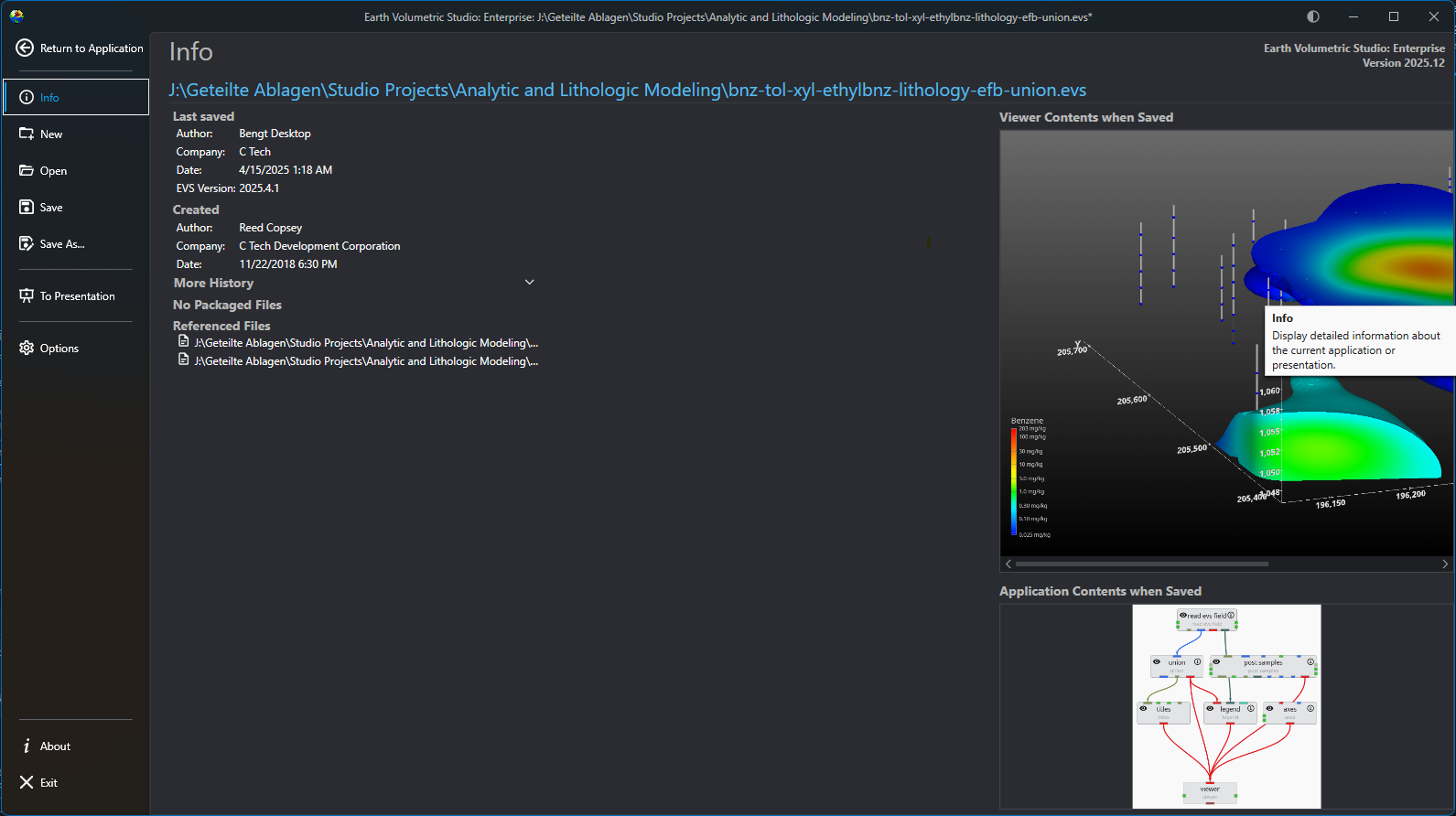
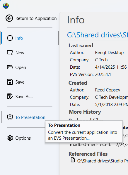
The main application menu serves as the central hub for managing your projects and configuring the application. Opening this menu will temporarily replace the standard workspace, including the Application Network and viewers, with a dedicated interface for file management, options, and project oversight. The Menu defaults to the Info screen, which provides an at-a-glance summary of your current project’s metadata and saved state.
Accessing the Menu
To open the menu, click the Show Menu button in the Main Toolbar.
Menu Screens
The navigation bar on the left side of the menu allows you to switch between several screens, each with a specific function.
Option
Description
Return to Application
Located at the top of the navigation bar, this button closes the menu and takes you back to your main workspace.
Info
The default screen, which serves as a dashboard for your current project. It displays important metadata (author, save date, version, etc.) and shows preview images of the Viewer Contents and Application Contents from the last save.
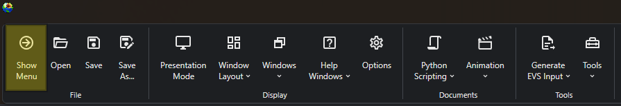
Opening Projects The Open screen, accessible from the main application Menu, provides a comprehensive interface for loading existing projects. It is designed to give you quick access to your recent work, sample files, and any project on your system, complete with metadata and visual previews to help you find the right file quickly.
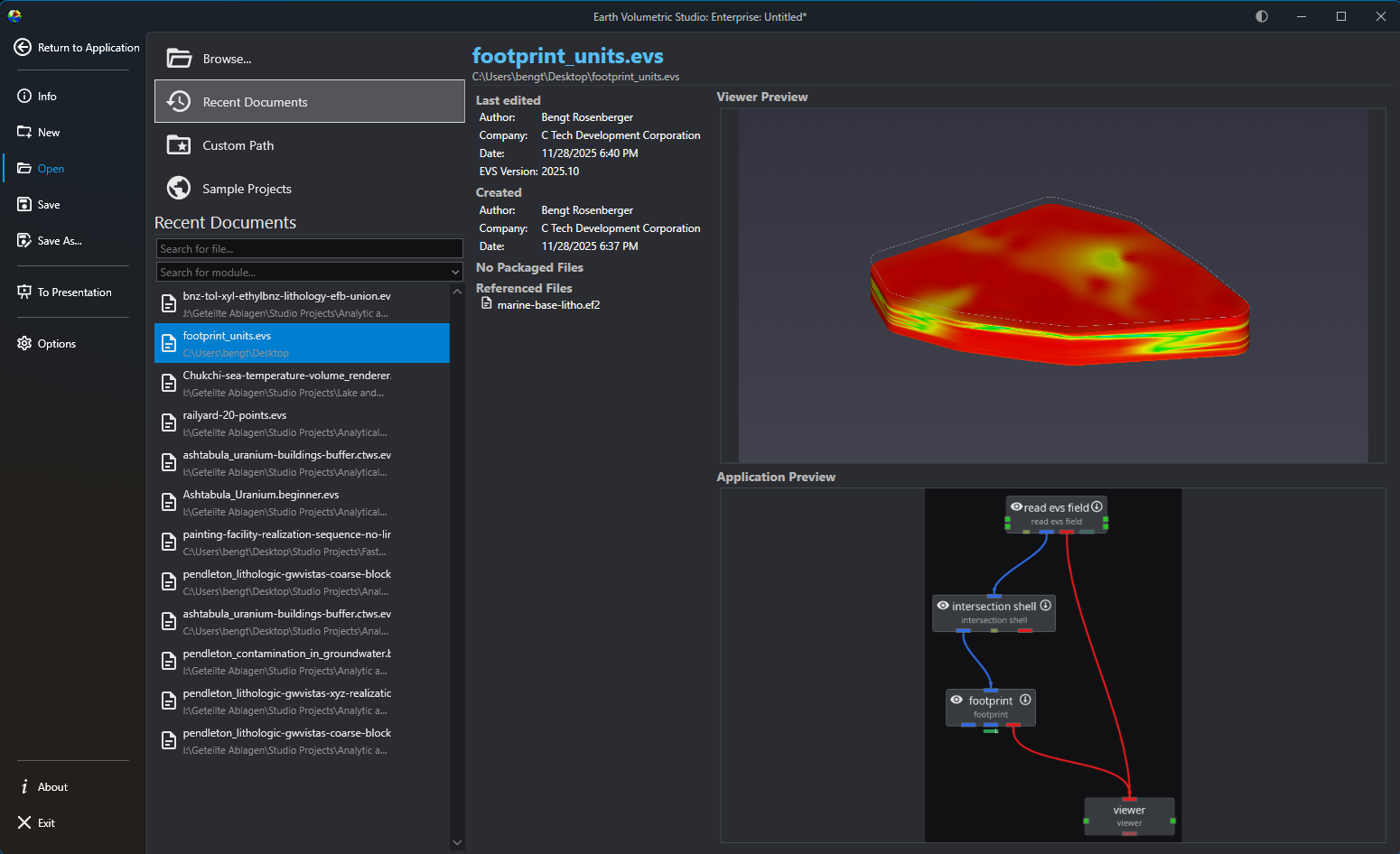
The Operation and User Preferences window is the central hub for configuring application-wide settings in Earth Volumetric Studio. It allows you to customize the user interface, set default behaviors for new projects, manage system resources, and personalize user information. Tailoring these settings can significantly improve your workflow and efficiency.
To access this window, click the Options button on the main application menu located on the left side of the screen.
Earth Volumetric Studio features a flexible interface composed of several windows. You can customize their size, position, and docking state to create
Subsections of Menu
Opening Projects
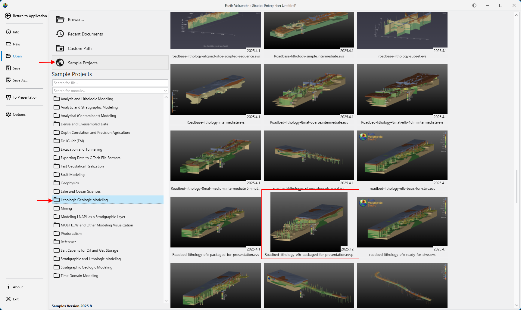
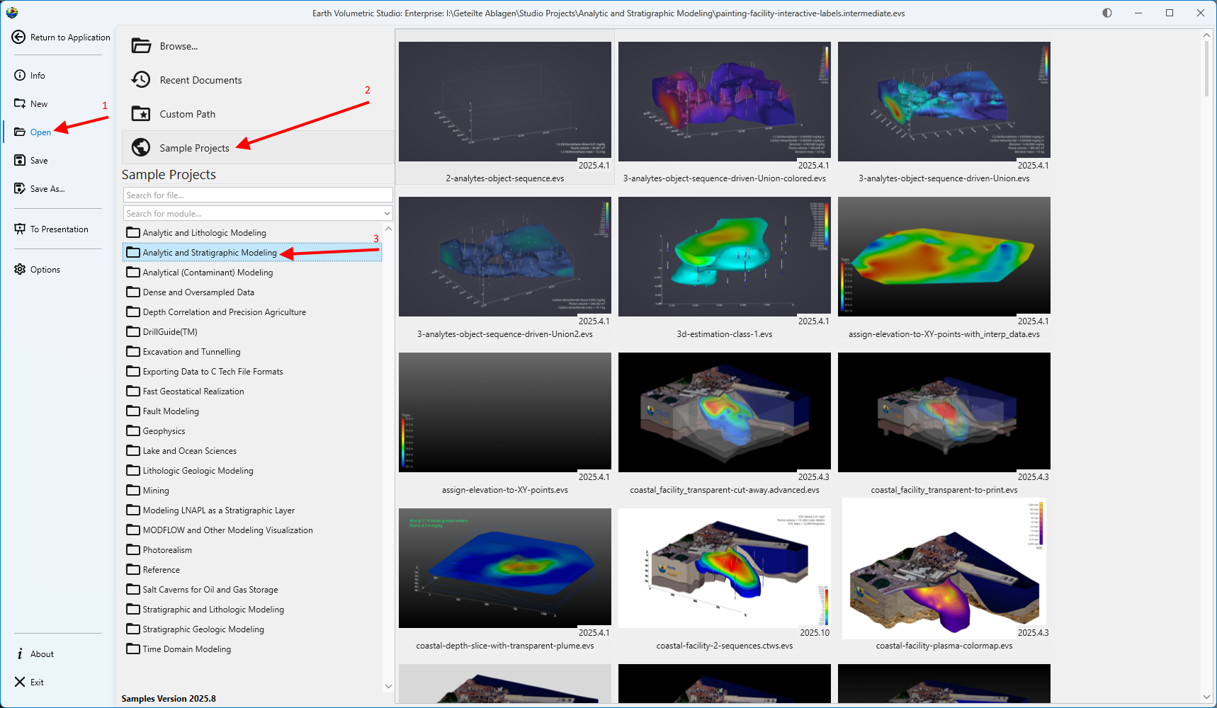
The Open screen, accessible from the main application Menu, provides a comprehensive interface for loading existing projects. It is designed to give you quick access to your recent work, sample files, and any project on your system, complete with metadata and visual previews to help you find the right file quickly.
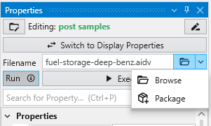
File Access Options
Option
Description
Browse…
Launches your operating system’s standard file explorer, allowing you to navigate your entire file system (local drives, network locations, etc.) to locate and open any .evs project file. This is ideal for accessing files not in your recent list or usual project folders.
Info
While applications on network drives or shared drives may load, our customers often experienced file locking or similiar access issues when saving them. For the best experience, we recommend loading applications from a local filesystem if possible.
|
| Recent Documents | The default view, offering the quickest way to resume work. It presents a scrollable and searchable list of your most recently accessed projects, ordered from newest to oldest. |
| Custom Path | Acts as a configurable bookmark for frequently used folders. Once you set a directory in the application’s options, this button lists all application files in that location, saving you from navigating to it manually.
Note: The Custom Path option will not recurse subdirectories. Only application files directly in the favorited directories will be shown. |
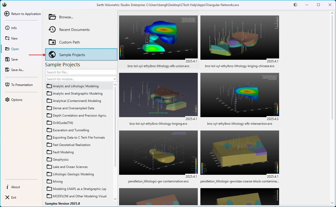
| Sample Projects | Provides access to a curated collection of official C Tech sample applications that demonstrate best practices and diverse capabilities. These are the applications used in the EVS Training tutorials.
Note: If this list is empty, the C Tech Sample Applications have not been installed. You can obtain the installer from the C Tech website at www.ctech.com. |
Filtering and Searching
When using the open file views, you can use the search and filter boxes to quickly locate a specific project. These tools are especially useful when dealing with a long list of files.
Tool
Description
Search for file…
This text box allows you to filter the list by filename. As you type, the list dynamically updates to show only the files whose names contain the text you have entered.
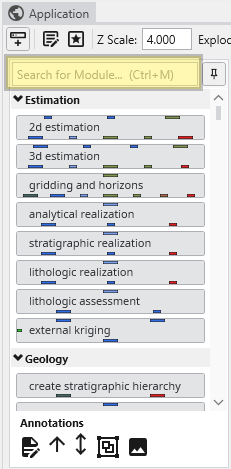
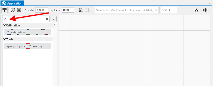
Search for module…
This dropdown helps you find projects based on their content. Selecting a module type will filter the view to show only application files containing that module. This is useful for finding examples or projects when you remember a key component but not the file name.
Project Information and Preview
When you select a file, the right-hand side of the screen populates with detailed information about that project.
Panel
Description
Metadata Panel
At the top, you will find key details about the file. This includes when it was last edited and by whom, its creation date, the software version used, and (for applications saved in recent releases) a list of any external files it references and any packaged data in the application.
Viewer Preview
This panel displays a static image of the 3D viewer’s contents as they appeared the last time the project was saved. This gives you an immediate visual reminder of the project’s output.
Application Preview
Below the viewer preview, a snapshot of the application network is shown. This allows you to see the module layout and connections, providing insight into the project’s workflow and structure.
The Operation and User Preferences window is the central hub for configuring application-wide settings in Earth Volumetric Studio. It allows you to customize the user interface, set default behaviors for new projects, manage system resources, and personalize user information. Tailoring these settings can significantly improve your workflow and efficiency.
To access this window, click the Options button on the main application menu located on the left side of the screen.
The window is divided into several logical sections, each handling a different aspect of the application’s configuration.
The options on the left side are all user preferences, and determine the look, feel, and operation of EVS for the current user. The options on the right side change the default values used for new modules and applications.
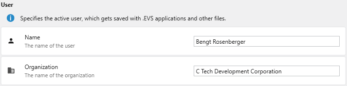
User
This section specifies the active user and their organization. This information is saved with .evs application files and other outputs, helping to track authorship and ownership of projects.
Setting
Description
Name
The name of the primary user. This name is stored as metadata within your project files.
Organization
The name of your company or organization. This is also saved as metadata for project management and collaboration.
System
The System section controls settings that impact the core operation of EVS system-wide, including file handling, hardware utilization, and integration with external tools like Python.
Setting
Description
Open EVS Files With Existing Instance
When enabled, any .evs file you open from Windows File Explorer will launch within the currently running instance of Earth Volumetric Studio. If disabled, a completely new instance of the program will be launched for each file.
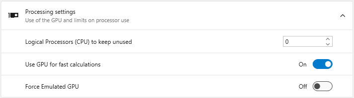
Processing settings
This section allows you to manage how EVS utilizes your computer’s hardware.
**Logical Processors (CPU) to keep unused**: Reserves a specific number of your CPU's logical processors (cores/threads) for the operating system and other applications. This prevents EVS from consuming 100% of your CPU during intensive calculations, keeping your system responsive.
**Use GPU for fast calculations**: When enabled, EVS leverages your graphics processing unit (GPU) to accelerate certain calculations. It is recommended to keep this enabled if you have a dedicated graphics card.
**Force Emulated GPU**: An advanced troubleshooting setting. It forces EVS to use a software-based GPU emulator instead of your physical graphics card, which can help diagnose graphics-related issues but at a significant performance cost.
|
| **Use Custom Python Installation** | Enable this toggle to use a specific Python installation on your system, rather than the one bundled with EVS.
NOTE: A restart of EVS is required for this change to take effect. |
| **Custom Python Install** | When "Use Custom Python Installation" is enabled, this field becomes active. Specify the path to the root directory of the desired Python installation. EVS must be restarted after changing this path. Any Python 3.10-3.13 installation will be detected and work, including Anaconda and similar (provided they are registered as a system Python install). Do not use Microsoft Store installed Python installations, as they are not allowed by Windows to be used by other software packages directly. |
| **Culture** | Specifies the language and regional format used throughout the EVS user interface, which affects language as well as the display of dates, times, and numbers. |
| **Custom Paths** | Define shortcuts to frequently used folders. These paths will appear directly in the **Open** menu and other file browsers, allowing you to navigate to project directories with a single click.
 |
User Interface Options
This section controls the visual appearance and layout of the EVS user interface.
Setting
Description
Theme
Choose a visual theme for the application. For more details, see the Themes topic.
Light: A bright theme with dark text.
Dark: A dark theme with light text, which can reduce eye strain.
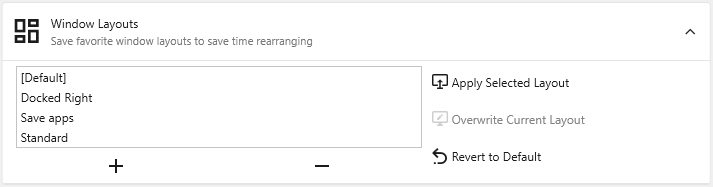
**+ / - Buttons**: Save the current window arrangement as a new layout or delete the selected layout.
**Apply Selected Layout**: Applies the window positions from the selected layout.
**Overwrite Current Layout**: Updates the selected layout with the current arrangement of windows.
**Revert to Default**: Resets the selected layout to its original state.
|
| **Ribbon Style and Density** | Customizes the appearance of the [Main Toolbar](../../main-toolbar/).
**Full Size**: The default style, featuring large icons with descriptive text.
**Comfortable**: A more compact style with smaller icons and text.
**Compact**: A minimal style with icons only.
**Display in Title Bar**: Moves the toolbar into the application's title bar to maximize vertical space.
|
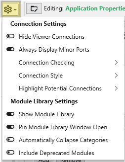
| **Application Window Options** | Controls the visual complexity and behavior of module connections in the [Application](../../the-application-window/) window.

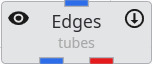
**Hide Viewer Connections**: Hides connection lines to and from Viewer modules to reduce visual clutter.
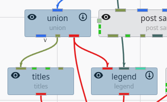
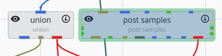
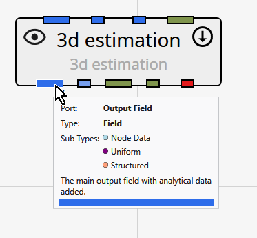
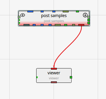
**Always Display Minor Ports**: When enabled, all module ports are visible. When disabled, less-used "minor" ports are hidden until you hover over the module.
**Connection Checking**: Determines how strictly EVS validates module connections. "Strict Checking" ensures data types are perfectly compatible.
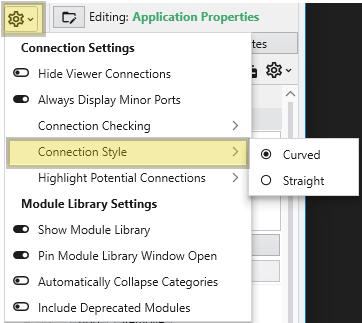
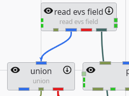
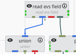
**Connection Style**: Sets the visual style of connection lines (Curved or Straight).
**Highlight Potential Connections**: Controls which available ports are highlighted as valid targets when dragging a connection (Major Ports Only, Include Minor Ports, or None).
**Max Potential Connections**: Limits the number of potential connections highlighted at once to maintain performance.
|
| **Properties Window Options** | Customizes the behavior of the EVS Properties Window.

**Display Expert Properties**: Reveals advanced or less commonly used module parameters.
**Always Show Critical Properties**: Ensures that important parameters are always visible, even if their category is collapsed.
**Automatically Collapse Categories**: When enabled, all property categories collapse when you select a new module.
|
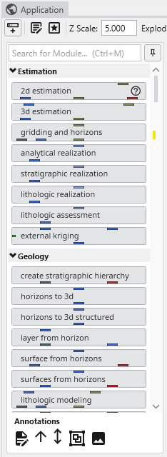
| **Module Window Options** | Options specific to the EVS [Module Library](../../the-application-window/module-library/) window.

**Include Deprecated Modules**: Shows older modules kept for backward compatibility.
**Automatically Collapse Module Categories**: When enabled, all module categories in the Module Library will be collapsed by default.
|
New Module and Application Default Settings
This area defines the default settings that are applied to new applications, modules, and data processing tasks.
New Application Defaults
Setting
Description
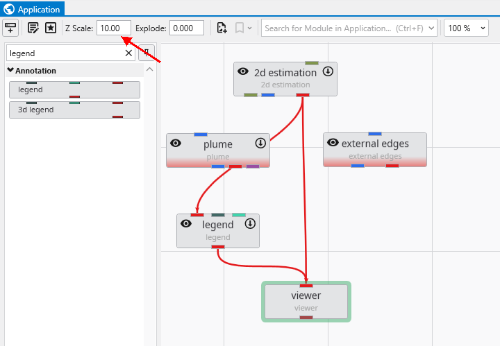
Z Scale
Sets the default vertical exaggeration (Z-Scale) for new applications.
Explode
Sets the default explode factor for new applications, which pushes modules apart in the 3D viewer.
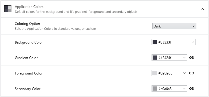
Application Colors
Sets the default colors for elements in the Viewer window for new applications.
**Coloring Option**: Select from predefined color schemes (Light, Dark) or choose "Custom" to enable the color pickers below.
**Background Color**: Sets the solid background color of the Viewer.
**Gradient Color**: Creates a two-color vertical gradient with the Background Color.
**Foreground Color**: Defines the default color for text, axes, and other primary annotations.
**Secondary Color**: Defines the default color for less prominent visual elements.
|
Module Defaults
Setting
Description
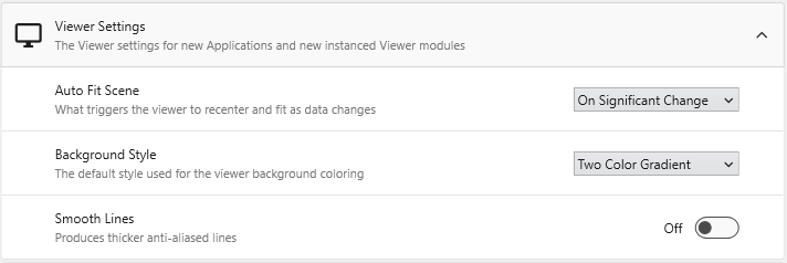
Viewer Settings
Defines the default rendering and behavior for new Viewer modules.
**Auto Fit Scene**: Controls when the viewer automatically rescales to fit all objects (On Significant Change, On Any Change, or Never).
**Background Style**: Sets the default background rendering style (Two Color Gradient, Solid, or Vignette).
**Smooth Lines**: When enabled, applies anti-aliasing to produce thicker, smoother lines.
|
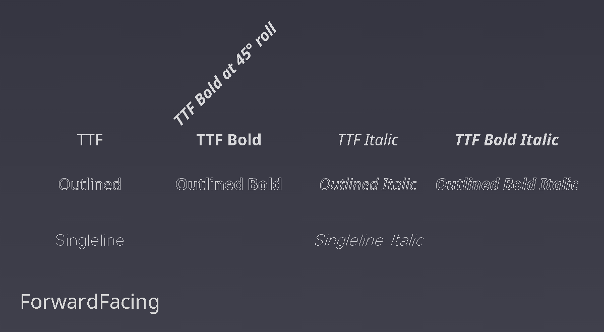
| **Text and Font Settings** | Controls the default font settings for new modules that display text.

**Default Font**: Sets the default font family for text in new modules.
**Force True Type Fonts**: When enabled, forces modules to use scalable TrueType fonts.
**Include Language Specific Fonts**: Loads additional font sets for displaying characters from non-Latin languages (e.g., Chinese, Japanese, or Korean).
|
Model Generation Defaults
Provides fine-grained control over the default parameters used in modules for gridding, data processing, and statistical estimation.
Setting Area
Description
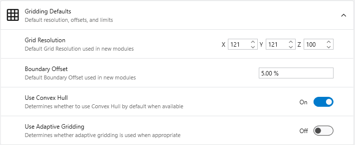
Gridding Defaults
Defines the default settings for new gridding modules like krige_3d.
**Grid Resolution**: Sets the default number of nodes in the X, Y, and Z dimensions.
**Boundary Offset**: Defines a default percentage to expand the grid boundary beyond the input data extents.
**Use Convex Hull**: When enabled, automatically uses the convex hull of the input data as the gridding boundary.
**Use Adaptive Gridding**: When enabled, uses adaptive gridding techniques by default.
|
| **Data Processing Defaults** | Changes the default data processing options in various modules.
**Pre Clip Minimum**: Sets the default minimum clipping value applied to data **before** interpolation.
**Post Clip Minimum**: Sets the default minimum clipping value applied to data **after** interpolation.
|
| **Estimation Defaults** | Defines the default parameters for estimation modules.

**Horizontal Vertical Anisotropy**: Sets the default ratio of horizontal to vertical anisotropy.
**Use all samples if # samples below**: When enabled, the module uses all data samples for estimation if the total count is below the specified limit.
**Number of Points**: Specifies the number of nearby data points to use for estimation.
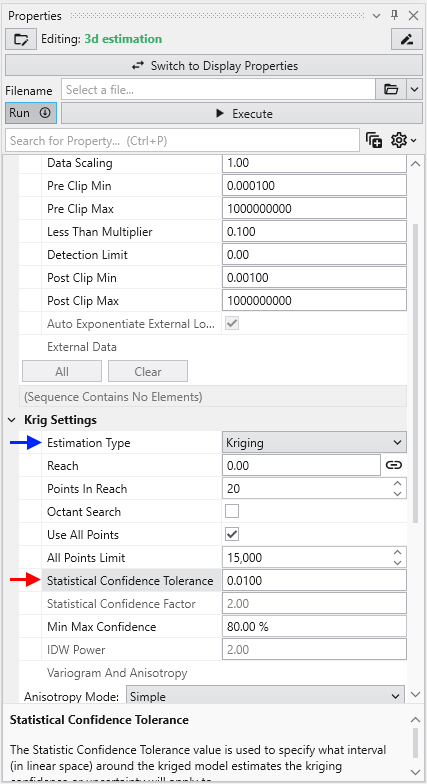
**Statistical Confidence Tolerance**: Sets the default tolerance for statistical confidence when data processing is "Linear".
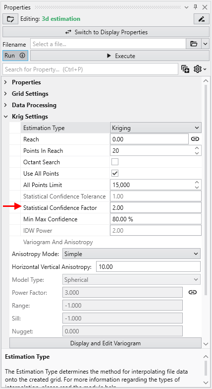
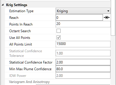
**Statistical Confidence Factor**: Sets the default factor for statistical confidence when data processing is set to "Log Processing".
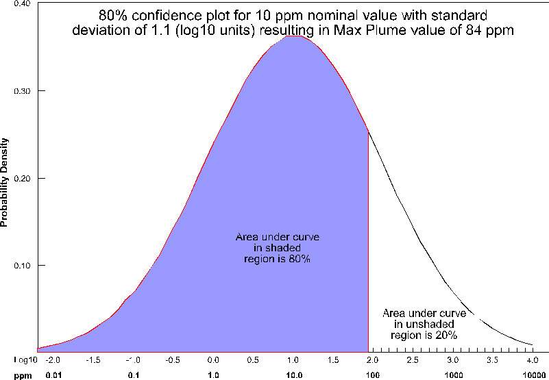
**Confidence for Min and Max Plume**: Sets the default statistical confidence level for determining plume extents.
|
Reset All Options
The Reset All Options button at the bottom of the window reverts all settings to their original factory defaults. This action is irreversible and affects all sections, so it should be used with caution.
Earth Volumetric Studio features a flexible interface composed of several windows. You can customize their size, position, and docking state to create a layout that suits your workflow.
Customizing Your Workspace with Window Layouts
EVS provides a flexible windowing system that allows you to customize the layout of your workspace. You can control the position, size, grouping, and visibility of most windows to suit your workflow. These customized layouts can be saved and reloaded, which is useful for different tasks or screen resolutions.
For example, here is an application with a personalized window layout:
Window Visibility and Docking
You can manage window visibility and docking using the controls located on each window’s title bar. While most windows can be moved, resized, or closed, there are a couple of exceptions:
Application Window: The main area for adding and connecting modules is always part of the main EVS application window, except in EVS Presentations or when working in Presentation mode.
Viewer Window: The Viewer cannot be closed, but it can be undocked and moved to another monitor for a multi-screen setup.
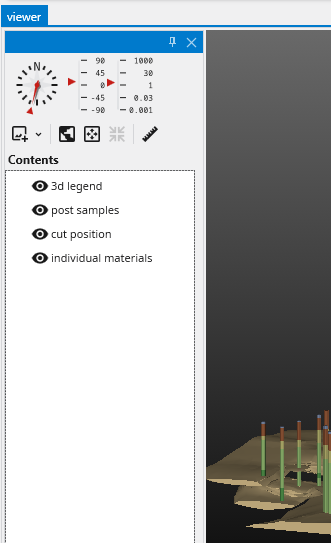
Example: Optimizing for a Larger Viewer
You can create different layouts to optimize your workspace. For instance, the layout below is configured to maximize the Viewer’s screen space. Notice how windows are tabbed together to save space:
The Application and Viewer windows are tabbed, with the Viewer active.
The Information, Packaged Files, and Output Log windows are tabbed, with the Output Log active.
Saving a Custom Window Layout
Once you have arranged the windows to your liking, you can save the layout for future use.
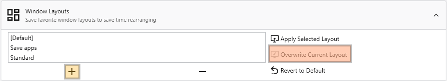
In the Options window, expand the Window Layouts section.
Here you have the option to create a new layout or overwrite the currently active layout.
Create a new layout: Click the + (Add) button to save your current window arrangement as a new layout. It will appear in the list along with any previously saved layouts and the “Default” configuration.
Overwrite the current layout: Click the Overwrite Current Layout button.
Loading or reverting a Custom Window Layout
There are two ways to switch to a different layout.
The Options window
You can load a previous or revert a layout in the same section as described above.
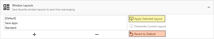
In the Options window, expand the Window Layouts section.
Here you have the option to load a layout or revert to the “Default” layout.
Load a layout: Select the desired layout and click the Apply Selected Layout button or alternatively revert to the “Default” layout using the Revert to Default button.
Revert to default: Click the Revert to Default button to revert the current layout to the one saved as “Default”.
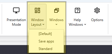
The Quick Access Button
You can easily switch between your saved layouts directly from the Main Toolbar.
Select your desired layout from the list to apply it instantly.
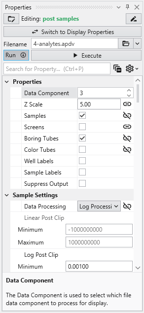
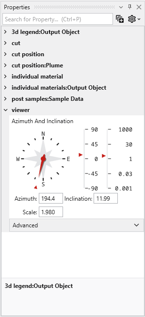
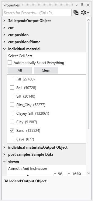
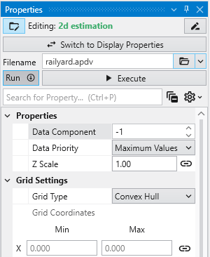
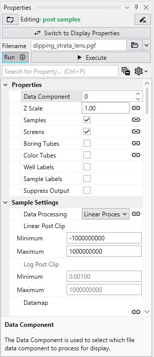
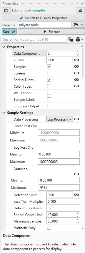
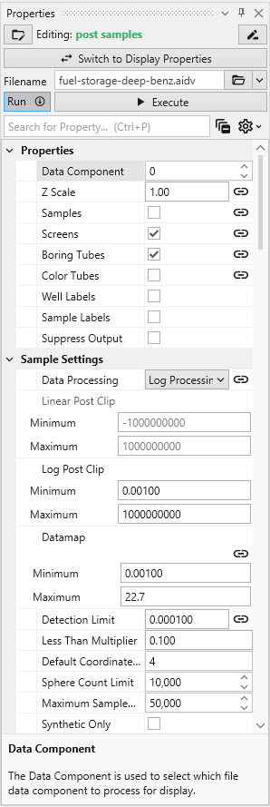
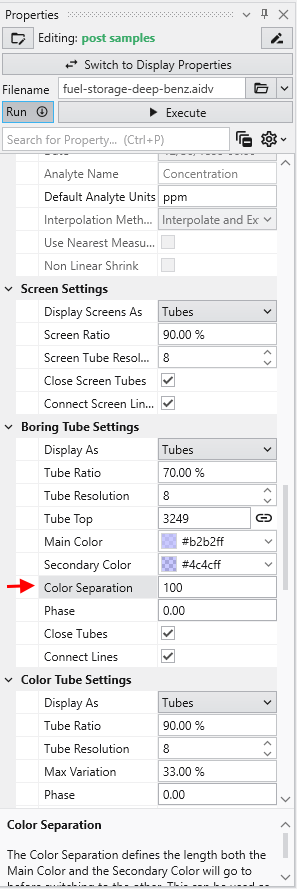
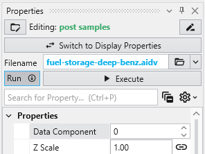
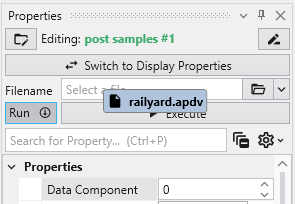
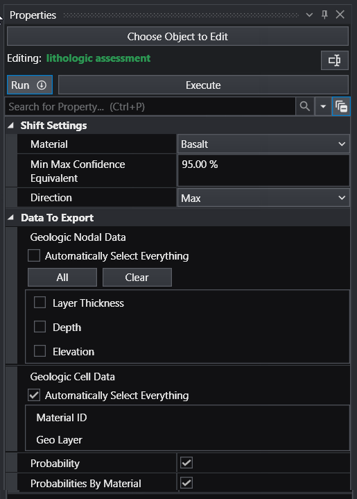
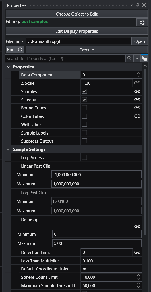
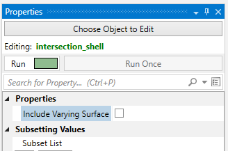
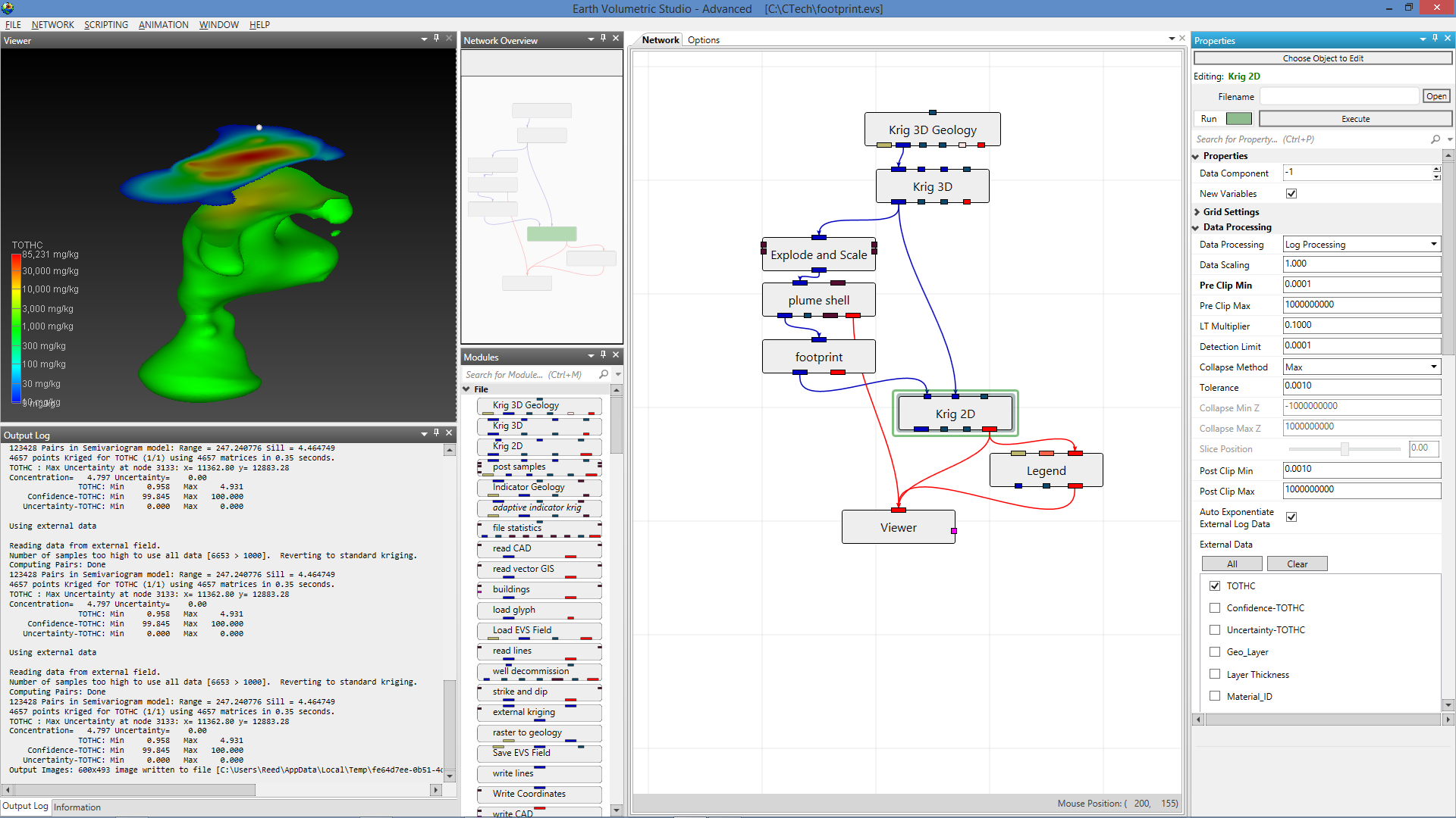
The Properties window is the primary interface in Earth Volumetric Studio for viewing and editing the parameters of various objects within your application. These objects can include modules, output ports, or the application itself. All properties for a selected object are displayed here, organized into logical, collapsible categories.
Module properties:
Application properties:
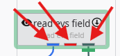
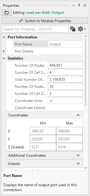
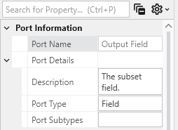
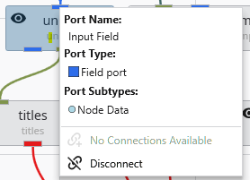
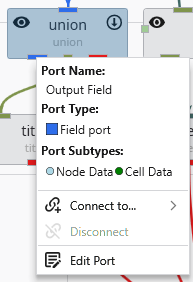
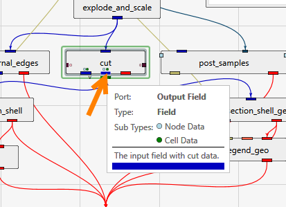
Port properties:
Accessing the Properties Window
If the Properties window is not already open, navigate to the Windows button in the Main Toolbar to show it.
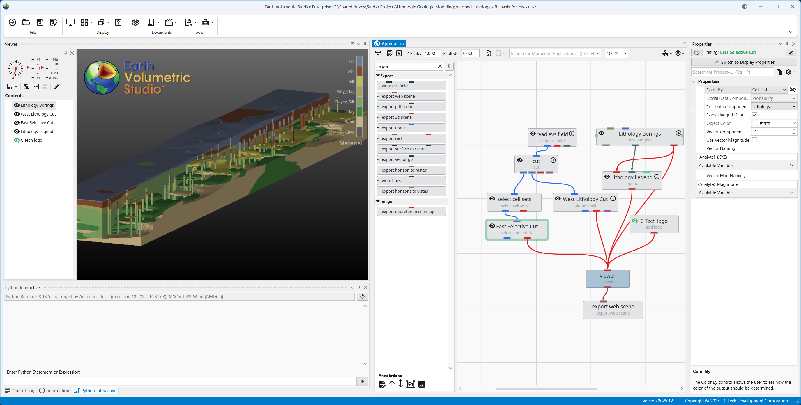
Editing Objects
Once the window is visible, you can load an object’s properties for editing. The most direct method is to double-click a module or a port of a module in the Application Network. Alternatively, you can use the Choose Object to Edit dropdown menu at the top of the Properties window, which provides a list of all objects in your application and allows you to quickly switch between them.
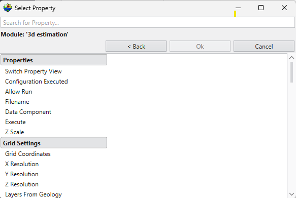
Navigating and Filtering Properties
The Properties window includes several tools to help you find and manage parameters efficiently. A Search for Property box at the top of the window allows you to filter the displayed properties by typing a search string; you can also use the Ctrl+P keyboard shortcut to focus on the search box. Next to the search box, the Collapse Categories button lets you expand or collapse all property categories at once.
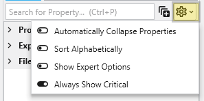
Options
Further customization is available through the Options menu, accessible via the gear icon. These are global settings for the Properties window and allow you to change how properties are displayed.
Option
Description
Automatically Collapse Properties
When enabled, all property categories are collapsed when properties of a new object are loaded.
Sort Alphabetically
Changes the order of properties to an alphabetical sorting.
Show Expert Options
Reveals advanced parameters.
Always Show Critical
Ensures essential properties are never hidden.
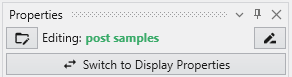
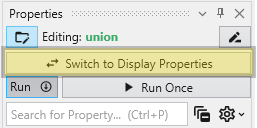
Toggling Module and Display Properties
The Switch to Display Properties button allows quick switching between the properties of the selected module and the properties of the primary red output port of it, if it has one. This is the same as double-clicking on the primary red port, but allows faster swapping right within the Properties window.
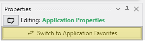
Toggling Application Properties and Application Favorites
The same button when shown in the Application Properties is labeled Switch To Application Favorites. It allows toggling between the two.
Property Descriptions
At the bottom of the Properties window is a description area. When you select a property from the list, this area displays a brief explanation of what the property does and how to use it, providing helpful context as you configure your modules.
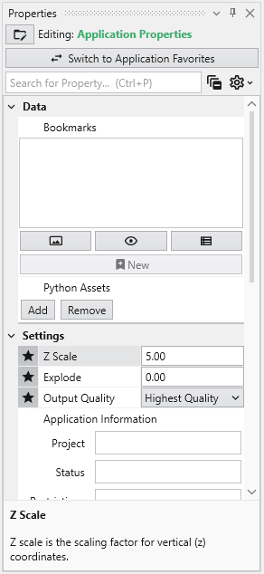
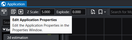
The Application Properties provide a centralized location to access critical parameters needed to control your application. Any property that impacts the application itself and is not specific to an instanced module will show here.
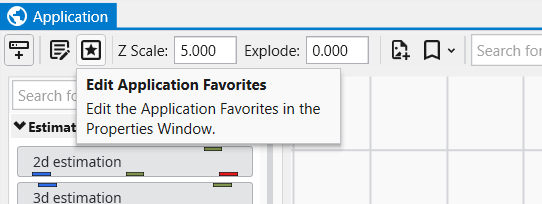
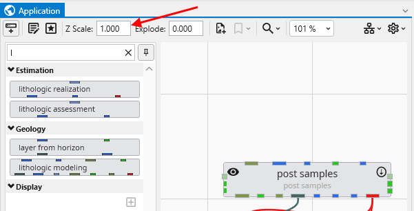
Accessing Application Properties The Application Properties are available via a button in the Application Window toolbar:
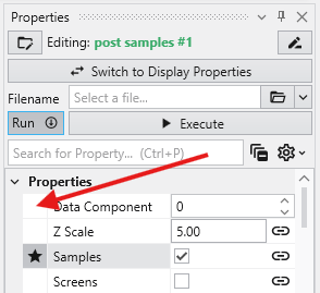
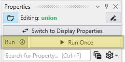
Module Properties When you select a module in the Application Network, its settings are displayed in the Properties window. This window allows you to configure the module’s parameters and control its execution behavior. At the top of the window, the name of the module you are editing is displayed.
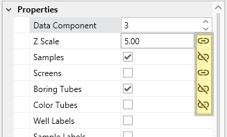
Understanding Linked Properties In Earth Volumetric Studio, a Linked Property is a parameter whose value is automatically determined within the application, rather than being manually set by the user. This dynamic connection allows for a more intelligent and consistent workflow. You can identify a linked property by the link icon located next to it in the Properties window
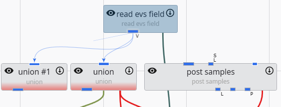
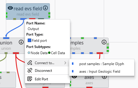
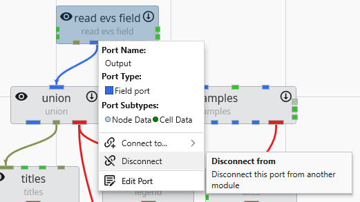
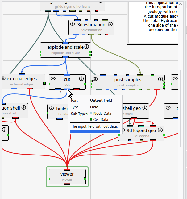
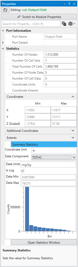
Port Properties When you double-click an output port on a any module in the Application Network, the Properties window displays detailed information and settings for that specific port. While the properties shown vary depending on the type of data the port provides, certain elements are common to all ports.
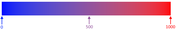
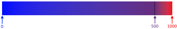
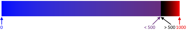
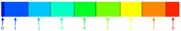
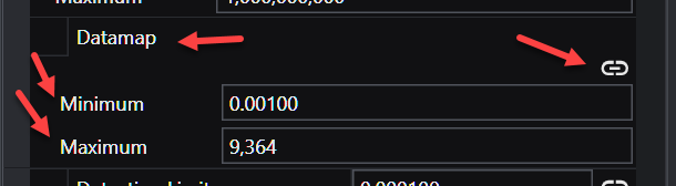
Introduction to Datamaps In the fields of scientific and geometric visualization, a datamap is a fundamental concept that serves as the bridge between raw numerical data and its visual representation. At its core, a datamap is a function or a lookup table that translates data values into visual properties, most commonly color. Think of it as a sophisticated legend that instructs the rendering engine how to “paint” the data onto a geometric object, such as a surface, a volume, or a set of points.
Subsections of Properties
The Application Properties provide a centralized location to access critical parameters needed to control your application. Any property that impacts the application itself and is not specific to an instanced module will show here.
Accessing Application Properties
The Application Properties are available via a button in the Application Window toolbar:
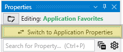
Alternatively, you can also access these when editing the Application Favorites. When the Application Favorites are displayed in the Properties window, click the Switch to Application Properties button at the top.
Finally, double clicking on the background of the network area will open the Application Favorites or Application Properties (whichever was most recently viewed).
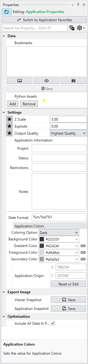
Available Application Properties
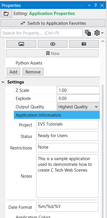
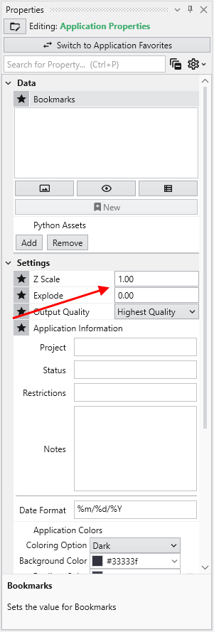
Below is the default content of Application properties.
Following is a description of each category:
Category
Property
Description
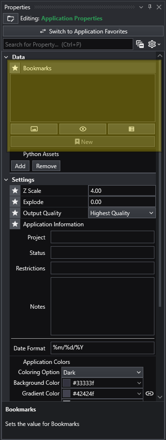
Data
Bookmarks
View and manage saved bookmarks. See Bookmarks for details.
Python Assets
Python scripts reusable from other Python files in your application. Right-clicking will generate the proper import syntax using the EVS python API, which allows these to be imported in scripts even when packaged.
Settings
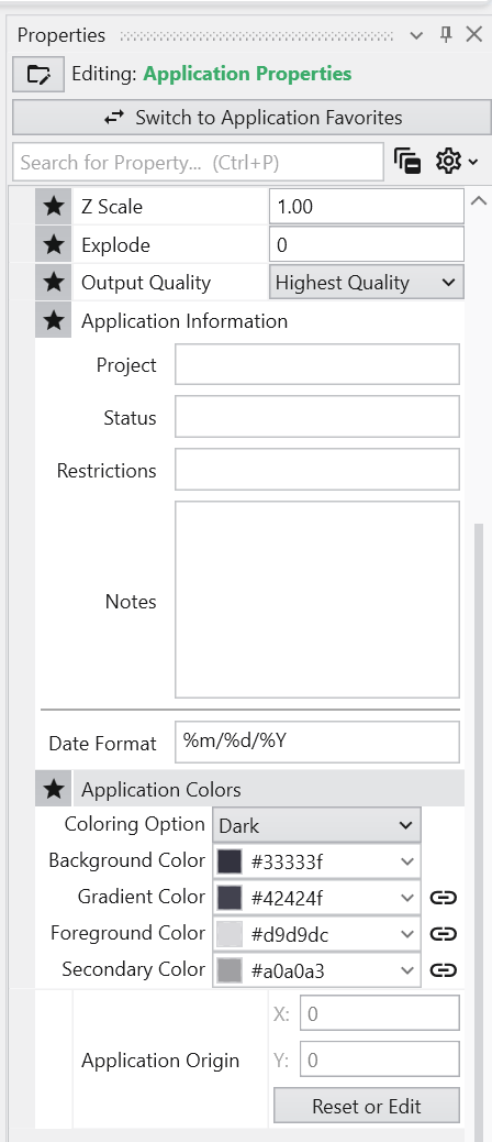
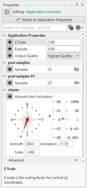
Z Scale
Adjusts the vertical exaggeration of 3D data.
Explode
Controls the separation of layered data components.
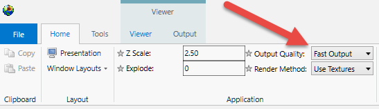
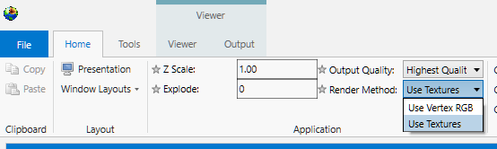
Output Quality
Set the quality setting used in certain modules (e.g., Highest Quality). Allows optimization of workflow by using a low quality file while manipulating and a high quality file when producing output.
Application Information
Provides a mechanism to supply reusable metadata in various outputs and scripts. Often available as environment variables in modules which produce text, as well as used in CTWS output.
Application Colors
Customize the appearance of many module outputs by default. See Application Colors for details.
Application Origin
Defines the spatial anchor for the project coordinates. The first time a file is read, the origin will be set based off the coordinates of that data. Everything is then computed relative to the application origin from then on in order to maintain the best precision for 3d calculations. If you reuse an application and change the data, you must reset the application origin.
Reset or Edit Origin
Allows manual recalibration of the project center.
Export Image
Viewer Snapshot
Writes the contents of the viewer to an image file.
Application Snapshot
Writes the contents of the application window (the network) to an image file.
Optimization
Include All Data In Probe
When enabled, all data is included in probe results in the viewer. This uses more memory, but increases the functionality for inspecting the data.
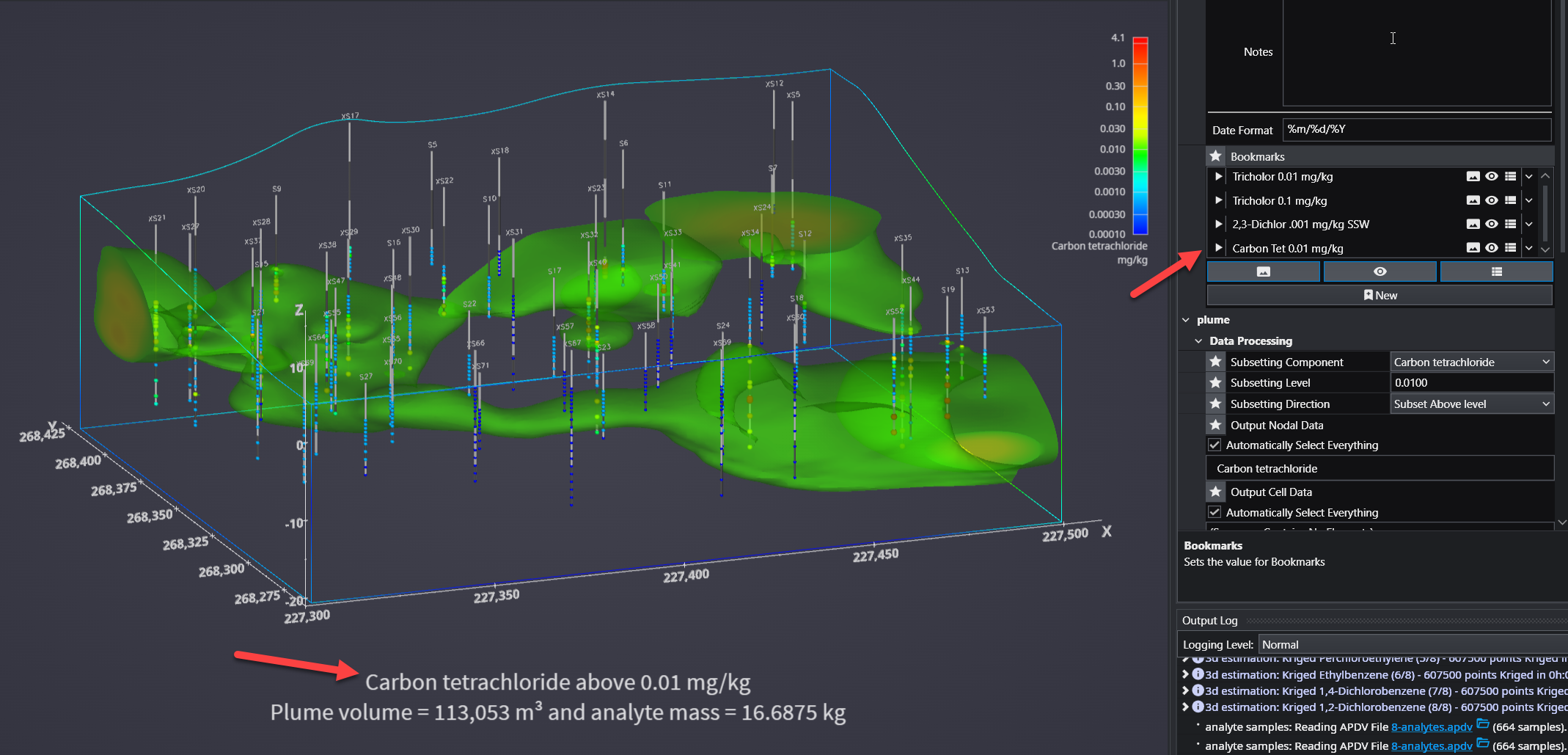
Bookmarks provide an easy way to save and recall specific configurations of your application. They act as saved “snapshots” that can instantly change the camera view, which objects are visible, and the current state of any sequences. They also export to C Tech Web Scenes.
This is essential for creating presentations, standardizing views for analysis, and optimizing the user experience in any exported C Tech Web Scenes.
The Application Colors feature provides a centralized way to manage a consistent color palette across your entire application. By setting a few base colors, you can ensure that various annotation modules - such as titles, legends, and axes - as well as the viewer background all share a coordinated and professional look.
This feature is particularly powerful when used with linked properties, as it allows you to switch between entire color themes (e.g., from a light to a dark theme) with a single click.
Subsections of Application Properties
Bookmarks provide an easy way to save and recall specific configurations of your application. They act as saved “snapshots” that can instantly change the camera view, which objects are visible, and the current state of any sequences. They also export to C Tech Web Scenes.
This is essential for creating presentations, standardizing views for analysis, and optimizing the user experience in any exported C Tech Web Scenes.
What Bookmarks Control
A single bookmark can be configured to control one, two, or all three of the following aspects of your application:
Aspect
Description
View
The camera’s position, orientation, and zoom level in the Viewer.
Visibility
The visibility and opacity settings of all modules in the application.
Sequence State
The currently selected state of all Sequence modules.
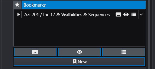
Bookmarks are created and managed from the Bookmarks panel in the Application Properties.
Follow these steps to create a new bookmark:
Set up your scene: Arrange the application to the exact state you want to save.
Adjust the camera to the desired view.
Set the visibility and opacity of each object in the Viewer.
Select the desired frame for any sequence animations.
Select Action Types: In the Bookmarks panel, click the buttons to activate the aspects you want this bookmark to control. The active buttons are highlighted in blue. From left to right, they are Views, Visibilities, and Sequence States. One or more of these must be selected to create a new bookmark.
Create the Bookmark: Click the New button (the plus icon). A new bookmark will appear in the list with a default name.
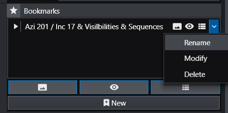
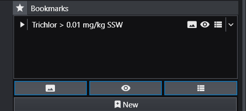
Rename the Bookmark: The default name can be generic. It is highly recommended to give it a descriptive name. Click the dropdown arrow on the far right of the bookmark and select Rename.
For example, a name like “Trichlor Plume > 0.01 mg/kg” is much more informative.
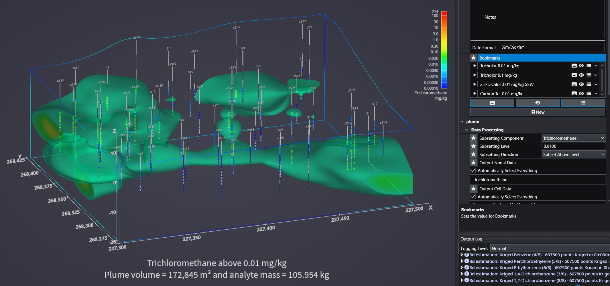
Using Bookmarks
To apply a bookmark, simply click the “Play” icon (the white triangle) next to the bookmark’s name in the list. This will instantly update the application to the saved view, visibility, and/or sequence state defined by that bookmark.
When you save your project as a C Tech Web Scene (.ctws file), these bookmarks are included, allowing others to interact with your scene in the predefined ways you have designed.
Advanced Visibility Options
When saving visibility in a bookmark, you have advanced control over how objects behave, which is especially useful for Web Scenes.
Option
Description
Locked
A “Locked” object is always visible and cannot be turned off by the user in the C Tech Web Scene Viewer. This is ideal for essential items like a site map, buildings, or a company logo that should always remain in view.
Excluded
An “Excluded” object is not written to the Web Scene at all. This is equivalent to disconnecting the module from the viewer and can be used to hide intermediate or unnecessary components from the final output.
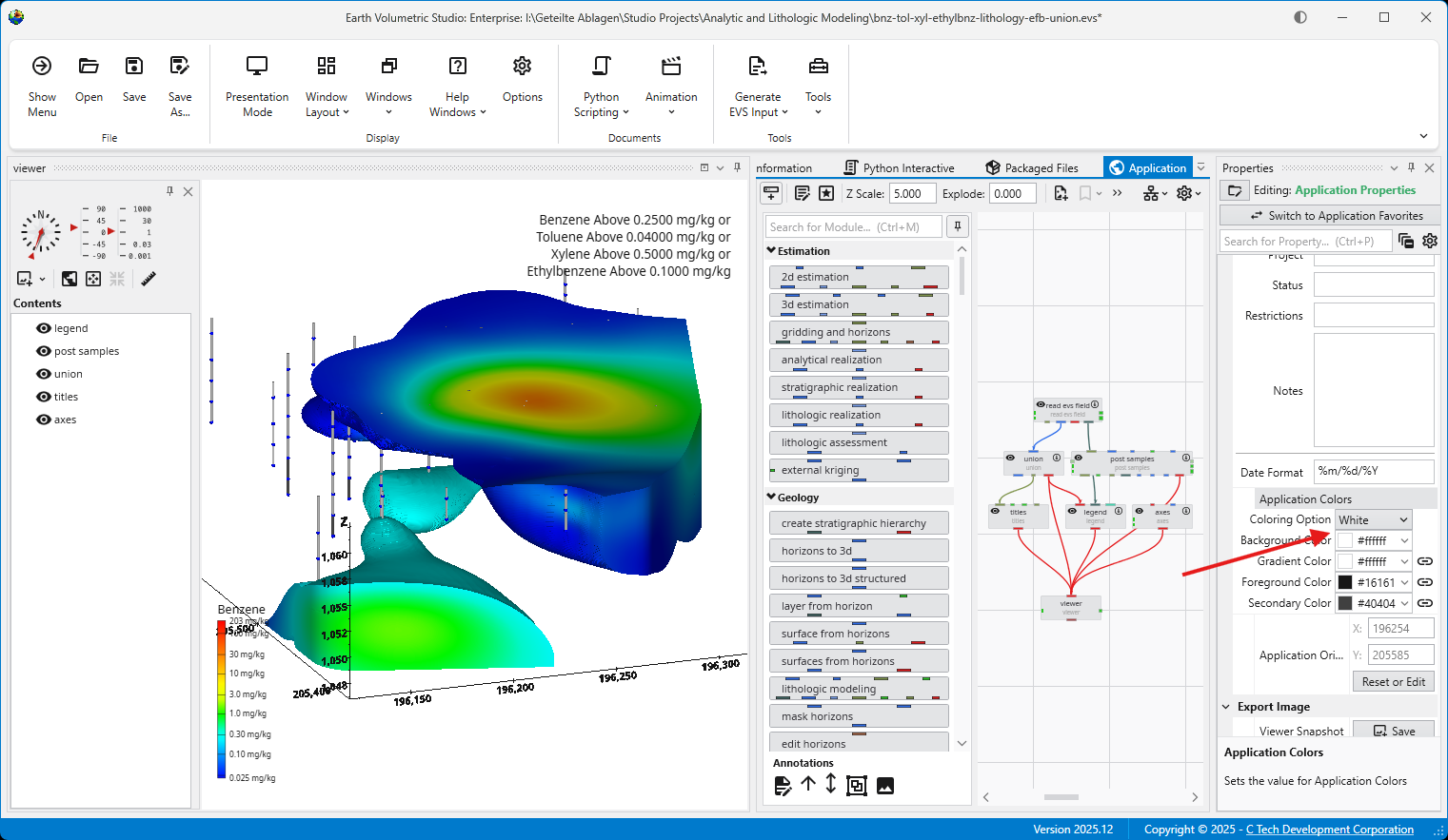
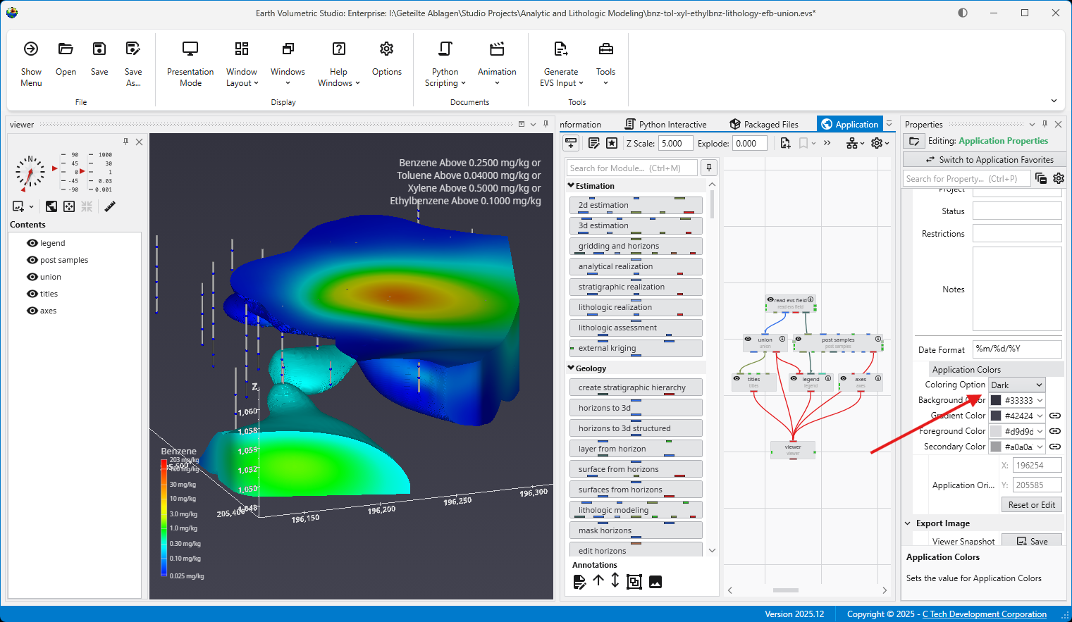
The Application Colors feature provides a centralized way to manage a consistent color palette across your entire application. By setting a few base colors, you can ensure that various annotation modules - such as titles, legends, and axes - as well as the viewer background all share a coordinated and professional look.
This feature is particularly powerful when used with linked properties, as it allows you to switch between entire color themes (e.g., from a light to a dark theme) with a single click.
Accessing Application Colors
The Application Colors settings are located in the **Application Properties**application-properties.md panel.
Color Properties and Options
The panel contains several options for defining your color scheme.
Option
Description
Coloring Option
This dropdown menu allows you to quickly switch between predefined color themes. By default, it includes “White” and “Dark” themes, which are designed for light and dark viewer backgrounds, respectively.
Interface Colors
These four properties define the core colors of your theme.
Background Color: Sets the background color of the viewer.
Gradient Color: Used with the Background Color to create a two-color gradient in the viewer background.
Foreground Color: The primary color used for text and lines in most annotation modules.
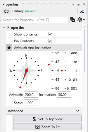
Secondary Color: A supplementary color used for secondary elements, such as shading on the compass rose in the direction_indicator module.
Linked Properties: The Key to Automatic Updates
For the Application Colors to automatically update your modules, the color properties within those modules must be linked. When a property is linked, it inherits its value from the global Application Colors settings. If you unlink a color property in a module, it will use its own manually set color and will no longer be affected by theme changes.
You can identify a linked property by the link icon next to it. For more information, see the Linked Properties topic.
Affected Modules
The following modules are designed to use the Application Colors when their color properties are linked:
Module
Usage
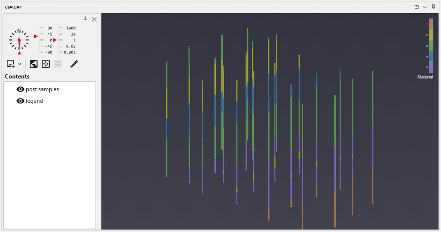
viewer
Uses the Background Color and Gradient Color for its background.
axes, titles, 3d_titles, legend, and 3d_legend
These modules primarily use the Foreground Color for their text and lines.
direction_indicator
This module uses the Foreground Color for its text and the Secondary Color for shading effects on elements like the compass rose.
Example of Switching Coloring Option
When the modules’ color properties are linked, changing the Coloring Option has an immediate effect on the entire scene.
The application below is using the White Coloring Option. Note the dark text and lines on the title, axes, and legend, which provide high contrast against the light background.
By simply switching the Coloring Option to Dark, all linked modules automatically update. The text and lines change to a light color to maintain contrast against the new dark viewer background.
Light and dark themes can also be toggled in the Options panel in the Menu.
The Application Favorites feature provides a powerful way to create a custom control panel for your EVS application. It allows you to gather the most important properties from various modules and global settings into a single, centralized location within the Properties window.
Info
When creating EVS Presentations, the only properties which will be editable in the resulting Presentation Application (*.evsp) are the Application Favorites. All other properties are unavailable in an EVS Presentation.
This is especially useful in large or complex applications, as it eliminates the need to navigate to each individual module to adjust key parameters. Instead, you can manage all critical settings from one convenient view.
Accessing Application Favorites
The Application Favorites are available via a button in the Application Window toolbar:
Alternatively, you can also access these when editing the Application Properties. When the Application Properties are displayed in the Properties window, click the Switch to Application Favorites button at the top.
Finally, double clicking on the background of the network area will open the Application Favorites or Application Properties (whichever was most recently viewed).
The Application Favorites View
Once you switch to the Application Favorites view, you will see a list of all the properties you have marked with a star. The properties are organized into groups based on their source module. For example, global settings like Z Scale and Explode are listed under “Application Properties,” while module-specific properties are grouped under the name of their respective module (e.g., “viewer”).
You can edit any of these properties directly from this view, just as you would in the standard properties editor.
How to Favorite a Property
You can favorite almost any property from any module.
Select a module in the Application Network to display its parameters in the Properties window.
To favorite a property, click in the empty space to the left of its name. A star icon will appear, indicating that the property has been added to your Application Favorites.
It is important to note that this action favorites the property for that specific instance of the module, not for all modules of that type. This allows you to select different key parameters from different modules. The same property from different modules can appear in the Application Favorites at the same time.
How to Remove a Property from Favorites
To remove a favorited property, simply click the star icon in either the module or the Application Favorites again.
Module Properties
When you select a module in the Application Network, its settings are displayed in the Properties window. This window allows you to configure the module’s parameters and control its execution behavior. At the top of the window, the name of the module you are editing is displayed.
Switch to Display Properties
This button provides a quick way to access the properties of the module’s primary Renderable Port (red) if they are being displayed in a viewer. The Red Port Properties will also feature a button to quickly switch back again.
Execution Control
The toolbar at the top of the Module Properties window provides powerful tools for managing when and how a module executes.
Run Toggle: This switch controls the module’s automatic execution. By default, it is on, meaning the module will automatically run whenever one of its properties is changed or when an upstream module it depends on finishes running. Toggling this off prevents the module from running automatically. This is particularly useful when you want to make multiple changes to a module’s settings without triggering potentially time-consuming computations after each adjustment.
This is also displayed and configurable on the modules in the Application Network. See Module Status Indicators.
Run Once Button: When available, this button allows you to manually trigger the execution of the currently selected module. It forces the module to run a single time. This is most effective when the Run toggle is turned off, as it lets you apply your changes and see the result without having to re-enable automatic execution.
Module-Specific Properties
Below the execution controls, the Properties section contains all the configurable parameters for the selected module. The settings here are unique to each module’s function. These properties allow you to customize the module’s behavior to fit the specific needs of your analysis.
Property Description
At the bottom of the Properties window is a description panel. This panel is your first and most important resource for understanding what a specific property does. When you select a property from the list, this panel automatically updates to show a detailed explanation of that property and its function. For instance, selecting “Data Processing” will display text explaining that this property allows to declare whether the input data is to be treated as linear or log processed. This immediate, context-sensitive help makes it easy to learn and configure even complex modules without having to consult external documentation.
Here is an example for the Property Description of the “Glyph Size” property:
Understanding Linked Properties
In Earth Volumetric Studio, a Linked Property is a parameter whose value is automatically determined within the application, rather than being manually set by the user. This dynamic connection allows for a more intelligent and consistent workflow. You can identify a linked property by the link icon located next to it in the Properties window
When the link icon is closed/connected, the property is linked, and its value will update automatically based on its source.
When the link icon is broken, the property is unlinked, and its value is fixed to whatever you have manually set.
You can toggle a property’s linked state by simply clicking on the link icon.
Linked Property:
Unlinked Property:
Info
Not all properties can be linked. If a property does not have a link icon next to it, it is a manual property. Its value may be set directly by the user and will not change automatically.
The Purpose of Linked Properties
Linked properties are a core feature of the EVS expert system, designed to streamline the modeling process. By linking properties, EVS can ensure consistency across your entire application, provide smart defaults based on your data, and maintain visual coherence. For example, linking the Z Scale of multiple modules to the global Application Z Scale means you only have to change it in one place, but can still unlink and override it as needed. Linked properties may also provide good automatic starting values for further unlinked manual refinement.
While you can unlink any linked property to gain manual control, it is generally recommended to keep properties linked unless you have a specific reason and understand the effect of the change. This approach leads to a faster and better-looking result.
Info
Re-linking a previously unlinked property will cause its value to revert to the automatic, context-driven setting. This change may also trigger the module to re-execute immediately to reflect the new state, unless the module’s Run toggle is turned off.
Common Categories of Linked Properties
Z Scale
This is the most common linked property and the one you should change least often. Nearly every module that deals with 3D data has a Z Scale property that is, by default, linked to the global Z Scale found in the Application Properties. This ensures that all visual components in your scene use the same vertical exaggeration, which is critical for correct spatial representation.
Colors
Many modules that create visual elements, such as titles or legends, have color properties that are linked to the global Application Colors setting. When you switch the application theme between Dark, White, or Custom, these linked colors will automatically adjust to ensure they remain visible and aesthetically pleasing against the new background color. Unlinking a color property, such as Title Color, will fix it to a specific color, and it will no longer adapt to theme changes.
Coordinates
Many modules that process spatial data have coordinate properties (e.g., Min/Max extents) that are linked to the incoming data. When the module is run, it analyzes the input field and automatically populates these properties with the correct coordinate values. If the input data changes, re-running the module will cause these linked properties to update accordingly.
Expert System Parameters
EVS includes an expert system that analyzes your data to provide intelligent, scientifically appropriate default values for complex parameters. This is most common in geostatistical modules like kriging or lithologic modeling. Parameters for kriging and variogram settings are often linked to the expert system, which suggests optimal values based on the input data. Unlinking these properties allows for manual fine-tuning but overrides the data-driven recommendations.
Port Properties
When you double-click an output port on a any module in the Application Network, the Properties window displays detailed information and settings for that specific port. While the properties shown vary depending on the type of data the port provides, certain elements are common to all ports.
At the top of the window, a Switch to Module Properties button provides a convenient way to navigate back to the properties of the module that owns the port.
Common Port Properties
All output ports display a Port Information section with the following properties:
Renderable Object Port Properties In Earth Volumetric Studio, a red port is a Renderable Object port. It outputs a visual object—such as a surface, a set of points, or a volume—that can be displayed in a viewer. By editing the properties of this port, you can control every aspect of how the object is visualized in the 3D scene. See the Visualization Fundamentals section for additional details on rendering options.
Field Port Properties In Earth Volumetric Studio, a blue port is a Field Port. It is the most common port type and is responsible for passing grid structures and their associated data between modules. A “field” contains the geometry (nodes and cells) as well as any data values defined on that grid, such as analytical results or material properties.
Subsections of Port Properties
Renderable Object Port Properties
In Earth Volumetric Studio, a red port is a Renderable Object port. It outputs a visual object—such as a surface, a set of points, or a volume—that can be displayed in a viewer. By editing the properties of this port, you can control every aspect of how the object is visualized in the 3D scene. See the Visualization Fundamentals section for additional details on rendering options.
To access these properties, you can double-click on a red port in the Application Network, which will load its settings into the Properties window.
Port Information
General information about the port as described in the Port Properties topic.
General Properties
This is the primary section for controlling the object’s appearance, coloring, and visibility in the 3D scene.
Property
Description
Visible
A master toggle to show or hide the object in the viewer.
Pickable
Determines if the object can be selected in the viewer using the probe tool (Ctrl + Left-click). Disabling this can be useful for large, transparent objects that might interfere with selecting objects behind them.
Opacity
Controls the transparency of the object. A value of 100% makes the object fully opaque, while 0% makes it completely invisible.
Faces To Display
Controls which faces of a 3D object are rendered.
Display All: Renders both the front and back sides of faces.
Camera Facing: Renders only the faces pointing toward the camera. This is useful for making closed transparent objects look correct and can improve performance.
Facing Away: Renders only the faces pointing away from the camera.
Color By
Determines the source of the object’s color.
Nodal Data: Colors the object based on data values at the nodes, often resulting in smooth color gradients.
Cell Data: Applies a uniform color to each entire cell based on its data value.
Solid Color: Applies a single, uniform color to the entire object.
Node Data / Cell Data
If coloring by data, these dropdowns let you select which specific data component to use for coloring.
Vector Component / Use Vector Magnitude
If the selected data is a vector, this allows you to color the object by a single component or by the vector’s overall magnitude.
Node/Cell Data Datamap
Opens the datamap editor to define the mapping between data values and colors. See the Datamaps topic for more information.
Object Color
If Color By is set to Solid Color, this control allows you to select the specific color for the object.
Object Secondary Color
This color is primarily used for drawing the outlines of cells when “Hide Cell Outlines” is disabled.
Normals Generation
Affects how lighting is calculated on surfaces.
Default: Selects the best method based on the input data type.
Cell Normals: Results in flat shading with hard transitions between cells.
Point Normals: Averages normals at each point, creating a smooth, continuous appearance.
Rendering Priority
A numeric value that influences the drawing order of objects. Objects with higher numbers are drawn later (on top of others).
Export Properties
This section contains settings related to exporting the application.
Property
Description
Exclude From Compression
If checked, this object’s geometry will not be compressed when exporting to a C Tech Web Scene. This preserves full precision but can result in a significantly larger file size.
Advanced Properties
These settings provide fine-grained control over geometry processing and rendering. They are intended for advanced users and should generally be left at their default values unless you are addressing a specific rendering issue.
Rendering Modes
This section controls how different geometric components of the object are displayed.
Property
Description
Point/Line/Surface/Volume/Bounds Display Mode
Each dropdown allows you to change the rendering style for a specific component (e.g., render a surface as a wireframe (Lines) or display points as spheres (Glyphs)).
Hide Cell Outlines
Toggles the visibility of the wireframe edges of the cells that make up the object.
Surface Properties
These properties control how the object’s surface interacts with light in the scene. They are intended for advanced users and should generally be left at their default values unless you are addressing a specific rendering issue.
Property
Description
Ambient
Controls how much ambient light the surface reflects (the object’s color in the absence of direct light).
Diffuse
Controls how much light the surface reflects from direct light sources, determining the primary illuminated color.
Specular
Controls the color of specular highlights (bright spots where light reflects directly toward the camera).
Gloss
Controls the size and intensity of specular highlights. Higher values create smaller, sharper highlights, making the surface appear shinier.
Point And Line Properties
This section contains settings that apply specifically to objects composed of points or lines.
Property
Description
Line Style
Sets the pattern for lines.
Solid: A continuous, unbroken line.
Dashed: A line made of a series of short segments.
Dotted: A line made of a series of dots.
**Dashed-Dotted: **A combination of the Dashed and Dotted line styles.
Line Thickness
Controls the width of lines in pixels. A value of 0 uses a default, fast-rendering single-pixel line.
Glyph Size
If points or lines are rendered as glyphs (e.g., quads), this controls their size.
Smooth Lines
Toggles anti-aliasing for lines. When enabled, lines will appear smoother with less jaggedness.
Texture Settings
If the object has a texture applied, these properties control how it is mapped and rendered. They are intended for advanced users and should generally be left at their default values unless you are addressing a specific rendering issue.
Property
Description
Interpolation
Determines how the texture is sampled when magnified or minified. Bilinear (default) averages the four nearest texels for a smooth but potentially blurry appearance.
Tile
Controls the texture’s behavior at its boundaries. Clamp causes the edge pixels to be stretched to fill the rest of the surface.
Blending
Defines how the texture’s color is combined with the object’s underlying color. Replace causes the texture’s color to completely overwrite the object’s original color.
Type
Relates to the use of mipmaps. Single Level indicates that only the original, full-resolution texture is used, without any lower-resolution versions for distant objects.
Field Port Properties
In Earth Volumetric Studio, a blue port is a Field Port. It is the most common port type and is responsible for passing grid structures and their associated data between modules. A “field” contains the geometry (nodes and cells) as well as any data values defined on that grid, such as analytical results or material properties.
To access the properties of a Field Port, you can double-click on any blue port in the Application Network. This will load its settings and summary information into the Properties window.
Port Information
General information about the port as described in the Port Properties topic.
Statistics
This section gives a high-level summary of the contents of the field.
Property
Description
Number Of Nodes
The total count of nodes (points) that define the field geometry.
Number Of Cell Sets
The number of distinct groups of cells. Cell sets are often used to represent different geologic layers or materials.
Total Number Of Cells
The total count of all cells across all cell sets in the field.
Number Of Node Data / Number Of Cell Data
The count of different data components attached to the nodes or cells.
Coordinate Units
The measurement unit for the grid’s coordinates (e.g., meters, feet).
Coordinate Extents
The overall dimensions (X, Y, Z) of the grid’s bounding box.
Coordinates
This table displays the minimum and maximum coordinate values for the X, Y, and Z axes, defining the spatial bounding box of the grid. The Z (Scaled) value reflects the coordinates after any global Z Scale has been applied.
Summary Statistics
This section provides a quick statistical overview of a selected data component within the field.
Property
Description
Data Component
A dropdown menu to select which data component you wish to analyze.
Data Units
The measurement unit for the selected data component.
Is Log
A checkbox indicating if the data is on a logarithmic scale.
Data Min / Data Max
The minimum and maximum values for the selected data component.
Histogram
A small histogram plot provides a quick visual summary of the data’s distribution.
Open Statistics Window
This button launches a separate, more detailed window for in-depth statistical analysis.
The Statistics Window
The Statistics Window provides a comprehensive and interactive environment for analyzing the data within a field. It is composed of several panels that allow you to customize the analysis and view detailed statistical results, both graphically and textually.
Panel / Component
Description
Analysis Settings
Located in the top-left corner, this panel allows you to control how the statistical analysis is performed and displayed.
Bin Count: Adjusts the number of columns in the histogram to change the granularity of the distribution plot.
Significant Figures: Controls the precision of the displayed numerical results.
Restrict Plot Range: When enabled, allows you to manually define the minimum and maximum values for the analysis.
Selected Component Statistics
Located below the analysis settings, this panel presents key statistical metrics for the chosen data component.
Data Mean: The average value.
Data Median: The middle value of the dataset.
Standard Dev.: The standard deviation, a measure of data dispersion.
Interquartile Rng.: The range between the first and third quartiles.
Histogram Plot
The main area on the right, providing a clear visual representation of the data’s distribution by showing the number of data values (Counts) that fall into each bin.
Statistics Summary
A text-based report below the plot, offering a summary of coordinate extents and a detailed breakdown of the statistics.
Bin Data Table
Located at the bottom, this table lists the specific data for each bin, including its minimum and maximum range, the count of values it contains, and the cumulative percentage of the total data set.
Introduction to Datamaps
In the fields of scientific and geometric visualization, a datamap is a fundamental concept that serves as the bridge between raw numerical data and its visual representation. At its core, a datamap is a function or a lookup table that translates data values into visual properties, most commonly color. Think of it as a sophisticated legend that instructs the rendering engine how to “paint” the data onto a geometric object, such as a surface, a volume, or a set of points.
Every value in your dataset, whether it represents temperature, contaminant concentration, pressure, or a geologic material type, is assigned a color based on the rules defined in the datamap. This transformation is what turns an abstract collection of numbers into an intuitive and immediately understandable visual model. Without datamaps, a 3D model of contaminant distribution would be a colorless, featureless shape, providing no insight into where the highest concentrations are or how they vary in space. The datamap is what brings the data to life, allowing us to see the patterns, trends, and anomalies that would otherwise be hidden in spreadsheets and data files.
The Purpose of Datamaps in EVS
In Earth Volumetric Studio, datamaps are the primary tool for communicating the meaning of your data within a visual context. Their purpose extends beyond simply making things colorful; they are a critical component of data analysis and presentation for several key reasons.
First, they make complex data interpretable. A bright red area in a plume model is instantly recognizable as a “hotspot” of high concentration, while a transition from green to blue can clearly show the gradient where values are decreasing.
Second, they provide a quantitative reference. A well-designed datamap, coupled with a legend, ensures that the visualization is not just a pretty picture but a scientifically accurate representation. Each color corresponds to a specific data value or range, allowing a viewer to probe any point on a model and understand its precise quantitative meaning.
Finally, they are essential for highlighting features of interest. Data in environmental and geological sciences often spans many orders of magnitude. A datamap can be carefully designed to focus the visual contrast on the most critical parts of the data range, making subtle but important variations stand out while de-emphasizing less relevant data.
Types of Data and Datamap Processing
Datamaps in EVS are highly flexible and can be configured to handle different types of data and distributions. The way a datamap translates values to color can be linear, non-linear, or categorical.
Linear Datamaps
A linear datamap applies a smooth, uniform color gradient across the entire range of the data. The relationship between a data value and its position in the color gradient is a straight line. For example, in a dataset ranging from 0 to 1000, a value of 500 would be mapped to the exact middle of the color ramp. This type of mapping is best suited for data that is evenly distributed and where the importance of changes is consistent across the entire range, such as a simple temperature scale.
Non-Linear Datamaps
A non-linear datamap is used when the data is not uniformly distributed or when certain ranges are more important than others. In this case, the relationship between data values and colors is not a straight line. This allows you to allocate more “color space” to the most critical parts of your data range.
A classic example is contaminant concentration data, which might range from 0.01 to 10,000. If a linear datamap were used, most of the color gradient would be dedicated to the high-end values, making it impossible to distinguish between low-level concentrations (e.g., 0.1 vs. 1.0), which might be the most critical range for regulatory purposes. A non-linear datamap can be configured to stretch the color gradient across the lower values, providing high visual contrast where it is needed most.
The colors of breaks on both sides don’t have to be continuous. If the Lock Adjacent Breaks toggle in the Datamap Editor is disabled, you can choose both colors separately.
A note on precision: Due to the nature of precision in floating-point calculations, a value that is identical to a break point can be categorized into either the adjacent upper or lower interval. If you need to ensure a specific value is colored correctly, we recommend slightly shifting the break point. For example, changing a break from 500.0 to 500.0001 ensures the value 500.0 falls into the lower interval.
Categorical Data
Datamaps are also used for categorical data, which is qualitative rather than quantitative. Examples include geologic material types (“Sand”, “Clay”, “Gravel”), land-use classifications, or sample location IDs. For this type of data, the datamap assigns a single, discrete color to each unique category. There is no gradient or blending between colors. In EVS, this is typically handled by assigning an integer ID to each category (e.g., Sand=1, Clay=2). The datamap is then configured with distinct colors for each integer value, effectively creating a color key for your categorical data.
Logarithmic Processing
Logarithmic processing is a specific type of non-linear mapping designed for data that spans several orders of magnitude. By taking the logarithm of the data values before mapping them to color, vast ranges are compressed into a more manageable scale. This makes logarithmic datamaps the standard and most effective way to visualize data like hydraulic conductivity or contaminant concentrations. EVS handles this transformation automatically when the log processing option is selected in many modules, so you do not need to manually convert your data. The datamap works with the log-transformed values, but associated legends will still display the original, human-readable values.
The Datamap Editor is the primary tool in Earth Volumetric Studio for creating and customizing the mapping between your data values and the colors used to represent them in a visualization. It provides a powerful, interactive interface to control color gradients, data ranges, and scaling, allowing you to effectively highlight the features of interest in your data.
Subsections of Datamaps
The Datamap Editor is the primary tool in Earth Volumetric Studio for creating and customizing the mapping between your data values and the colors used to represent them in a visualization. It provides a powerful, interactive interface to control color gradients, data ranges, and scaling, allowing you to effectively highlight the features of interest in your data.
You can access the Datamap Editor by clicking the Edit button next to the Node Data Datamap or Cell Data Datamap properties in a module’s rendering settings.
The editor is composed of three main areas: the toolbar at the top, the color ramp preview in the middle, and the color break editor at the bottom.
Toolbar
The toolbar provides access to file operations, settings, and tools for manipulating the datamap.
File and Replace Operations
Operation
Description
Open
Allows you to load a previously saved datamap configuration from a .CTDmap file, enabling you to reuse complex color schemes across different projects and models.
Save
This dropdown menu provides two distinct ways to save the current datamap configuration to a .CTDmap file.
Save As Generic: Saves the datamap with its breaks defined by their relative positions (e.g., percentages). This makes the saved datamap a flexible template that will adapt to a new dataset’s minimum and maximum values.
Save With Values: Saves the datamap with its breaks locked to their current, fixed data values. This is useful for applying a consistent color mapping to multiple datasets that share the same data extents or have specific, meaningful thresholds.
Use Template
Applies one of the default datamap templates, such as Default Node Map, Linear Grayscale, or perceptually uniform scientific colormaps.
Copy From
Opens a dialog to copy a datamap from another module in your application, allowing you to select a specific source and apply its datamap to the current module.
Copy To
Performs the reverse of Copy From. It allows you to apply the current datamap’s configuration to one or more selected modules and ports.
Settings
Setting
Description
Lock Adjacent Breaks
This toggle locks the colors between breaks. When enabled, changing the color of a break point will also update the adjacent break point in the next range, ensuring a continuous color gradient.
Gradient Color Ranges
This toggle controls whether to use smoothly changing colors. When enabled, colors blend seamlessly between break points. When disabled, each range is filled with a single, solid color.
Use Perceptual Colorspace
This option switches the color interpolation method to a “visual perceptual colorspace,” which can produce gradients that are perceived as more uniform and natural by the human eye.
Operations
Operation
Description
Add Break
Adds a new break position to the datamap, allowing you to introduce a new color and data value point to refine your color gradient.
Evenly Space Breaks
Redistributes all existing color breaks linearly across the full data range, creating a uniform gradient.
Clear Breaks
Removes all intermediate color breaks, leaving only the start and end points and creating a simple, two-color gradient.
Create Breaks From Bands
Automatically creates new color breaks at the exact data values used by another module (like isolines), ensuring color changes align perfectly with contour lines or other banded visualizations.
Flip Ranges
Reverses the color ramp, so that the color previously at the maximum value is now at the minimum value, and vice-versa.
Apply Geologic Mapping
Designed for categorical data, this function creates a series of discrete, solid color ranges corresponding to the integer IDs used to represent different geologic materials.
The toolbar also has similar options to the EVS Main Toolbar in terms of display style and density.
Color Ramp and Break Editor
This is the main interactive part of the editor where you define the datamap.
Color Ramp Preview: The large horizontal bar shows a preview of the final datamap. It displays the colors and the smooth transitions between them, based on the color breaks you have defined below it. The minimum and maximum data values of the current range are displayed at the ends of the ramp.
Logarithmic Scaling Indicator: Text such as “Logarithmic Scaling On” will appear to the right of the color ramp. This indicates that the datamap is currently processing the data on a logarithmic scale. This is essential for effectively visualizing data that spans several orders of magnitude, as it allocates more color variation to the lower-end values.
Color Break Editor: This section is where you define the specific points of your datamap. The datamap is composed of one or more color intervals, and the points that define the start and end of these intervals are called color breaks. Within each interval, the color transitions in a linear gradient based on the data values and colors set at its start and end breaks. A key feature of the editor is that the color at the end of one interval does not need to be continuous with the color at the start of the next. By disabling the Lock Adjacent Breaks setting, you can create a “hard break,” or an abrupt change in color at a specific data value. This is useful for visually separating distinct data ranges. Furthermore, the length of each interval can be adjusted independently, allowing you to create a non-linear datamap by stretching or compressing the color gradient across different parts of the data range.
Each color break is represented by a row in the editor, which includes:
Component
Description
Data Value Input Box
Allows for precise numeric entry of the data value for the break.
Color Swatch
Opens a color picker to set the color for the break.
Slider
Provides interactive adjustment of the data value for the break.
Delete Button
A trash can icon to remove the break.
The Application window is the central workspace in Earth Volumetric Studio for creating and managing your data processing and visualization workflows. It provides a visual, node-based environment where you build networks by placing and connecting modules to define a data flow.
The window is divided into two main sections: the Module Library on the left and the Application Network on the right.
Module Library
The Module Library contains a comprehensive list of all available modules, organized into categories such as Estimation, Geology, and Annotations. To build your application, you can find the desired module in the library and drag it onto the Application Network canvas.
This topic is discussed in more detail in the Module Library topic.
Application Network
The Application Network is the gridded canvas where you assemble your workflow. Modules are placed here and connected to one another to control the flow of data. Each module has input and output ports, and you create connections between matching ports on different modules. This visual representation allows you to easily understand and modify the data processing pipeline. The style of the connections (curved, straight) can be controlled in the Application Options.
A toolbar at the top of the Application window provides quick access to various tools and settings for managing your application.
Tool
Icon
Description
Show Module Library
Toggles the visibility of the Module Library panel on the left.
Edit Application Properties
Opens the Application Properties in the Properties window. These properties are global settings that apply to the entire application, such as Bookmarks and Colors.
Edit Application Favorites
Opens the Application Favorites in the Properties window. This panel contains a collection of all module properties that you have manually marked as favorites, providing quick access to them.
Z Scale
Controls the global vertical exaggeration for all viewers in the application.
Explode
Controls the global explode factor, which separates objects in the viewer for better visibility.
Create Snapshot
Saves a snapshot image of the current state of the Application Network.
Bookmarks
A dropdown menu that allows you to quickly toggle between saved bookmarks, which store specific camera views and other scene settings.
Provides controls to manage the zoom level of the Application Network. You can zoom in or out, reset the zoom to its default level, or automatically adjust the zoom to fit the entire network within the view.
Application Overview
Shows a stylized, high-level overview of your Application Network, which is useful for navigating large and complex applications. You can click on that overview to zoom in on that part in the Application Network.
Options Menu
The Options menu contains settings related to connections and the Module Library.
Connection Settings
Hide Viewer Connections: Toggles the visibility of connection lines leading to any viewer modules.
Always Display Minor Ports: When enabled, all module ports (both major and minor) are displayed. When disabled, only major ports are shown by default.
Connection Checking: Submenu for settings related to data type validation when connecting modules.
Connection Style: Submenu to change the appearance of connection lines (e.g., curved or straight).
Highlight Potential Connections: Submenu to control which ports a connection can connect to when you are creating a new connection.
Module Library Settings
Show Module Library: Toggles the visibility of the Module Library.
Pin Module Library Window Open: Keeps the Module Library panel open and prevents it from automatically collapsing.
Automatically Collapse Categories: If enabled, module categories are collapsed by default.
Include Deprecated Modules: Toggles the visibility of older, outdated modules in the Module Library.
The Module Library is a core component of the Application window, serving as the repository for all modules used to build data processing and visualization workflows. It is located on the left side of the Application window and a fixed part of it. Unlike most other windows, it cannot be undocked, but it can be hidden when not in use.
Finding Modules in the Application Network For large or complex application networks, the search functionality provides an efficient way to locate specific modules. The search tool is located in the toolbar at the top of the Application window.
Using the Search Tool The appearance of the search tool depends on the available width of the Application window. In narrower views, it may appear as a magnifying glass icon. In wider views, it will be displayed as a full search box labeled “Search for Module in Application”.
Subsections of Application
The Module Library is a core component of the Application window, serving as the repository for all modules used to build data processing and visualization workflows. It is located on the left side of the Application window and a fixed part of it. Unlike most other windows, it cannot be undocked, but it can be hidden when not in use.
Modules are organized into collapsible categories, such as Estimation and Geology, allowing you to easily browse and find the tools you need. You can control whether these categories are expanded or collapsed by default in the Options menu of the Application window. To add a module to your workflow, simply drag it from the library and drop it onto the Application Network canvas. Alternatively, double clicking a module will also create a new instance on the Application Network.
At the top of the Module Library, you will find controls for searching and docking.
The Search bar allows you to quickly filter the list of modules. As you type, the library will display only those modules whose names match your search query. You can also use the keyboard shortcut Ctrl+M to focus on the search bar, even if the Module Library is unpinned and closed.
Next to the search bar is the Pin button. This button controls the auto-hide behavior of the Module Library. When the library is pinned, it remains permanently visible. If you unpin it, the library will automatically slide away when not in use and can be reopened by clicking the Show Module Library button in the Application window’s toolbar or via the keyboard shortcut Ctrl+M.
Annotations
At the bottom of the Module Library is a set of tools for adding visual annotations to your Application Network. These elements help document your workflow, clarify connections, and organize complex applications. Clicking on an annotation shows contextual menu items such as Delete, Copy, Paste and a coloring option.
Annotation
Description
Text Annotation
Adds a text box directly onto the Application Network canvas. You can use it to add notes, titles, or descriptions for different parts of your workflow.
Line Annotations
There are two types of line annotations for drawing arrows on the canvas. These are useful for pointing to specific modules or visually grouping related items that may not be physically close to each other.
Group Annotation
Creates a visual container for a set of modules. You can drag modules inside a group annotation to organize them as a logical unit. The group can be named, resized, and collapsed, which can be useful for simplifying the view of a large Application Network. When you collapse a group, it is displayed as a single item, and all connections to the modules it contains are shown connecting to the group instead.
Image Annotation
Places an image from a file directly onto the Application Network canvas. This can be used for adding logos, diagrams, or other visual aids to your workflow documentation.
The Application Network is the primary workspace in Earth Volumetric Studio for building and managing your data processing workflows. It is a visual, node-based environment where you construct “applications” by placing modules and connecting them to define a data flow from input to final visualization.
Modules
Modules are the fundamental building blocks of an application. Each module performs a specific task, such as reading data, performing a calculation, creating a geometric object, or rendering a scene. They are represented by rectangles on the Application Network, each stating a user-defined name and the module type under it. You add modules to your network by dragging them from the Module Library onto the Application Network canvas.
Each module has a set of icons that appear when you hover over it, providing quick access to key functions:
Icon
Description
Disable/Enable Module
Clicking this icon disables the module and any downstream modules that depend on it. A disabled module will not execute when the application is run. The icon appearance will change to quickly notice disabled modules. Clicking the icon again re-enables it and will make it run immediately.
Hide/Show Output
This icon is available on modules that produce a visual output. Clicking the eye icon toggles the visibility of that module’s output in all viewers.
Modules communicate with each other through ports. Each module has one or more input ports (on the top) and output ports (on the bottom). You create Connections between modules which define the top-down Data Flow of the application, directing the output of one module to become the input for the next. See the Connecting and Disconnecting Modules topic.
Ports are color-coded to indicate the type of data they handle, and you can only connect ports of a similar color. While there are many port types, the two most critical and frequently used are Field ports and Renderable Object ports.
Connections can be removed by selecting the connection with the left mouse button in the Application Network and then either using the DEL key or by clicking the right mouse button and choosing the Disconnect option.
Module Right-Click Menu
Right-clicking on any module in the Application Network opens a context menu that provides quick access to several common actions and properties for that module.
Option
Description
Rename
Allows you to change the display name of the module as it appears on the Application Network canvas.
Edit
Opens the selected module’s parameters in the Properties window.
Copy
Creates a duplicate of the selected module, including its current settings. The new module can be pasted with CTRL+V.
Visible
This toggle, represented by an eye icon, controls the visibility of the module’s output in the viewer (applies only to modules with a red output port).
Opacity
This slider and input box allow you to adjust the transparency of the module’s visual output in the viewer.
Position
Displays the read-only X and Y coordinates of the module’s top-left corner on the Application Network canvas.
Delete
Removes the module and all of its connections from the Application Network.
Input Port Context Menu
Right-clicking on a module’s input port opens a context menu providing details and actions for the incoming connection.
Option
Description
Port Name
Displays the name of the port.
Port Type
Shows the type of data the port accepts, indicated by a colored icon and a description.
Port Subtypes
Lists the specific kinds of data this port requires the output port to provide.
No Connections Available / Connect from…
Indicates if compatible output ports are available. If so, it allows you to create a connection.
Modules in the Application Network feature a set of icons directly on their surface that provide at-a-glance information and quick control over their execution and visibility. Modules that can be executed or produce a visible output have icons on their left and right sides. The right-side icon controls execution, while the left-side icon controls visibility in the viewer.
Modules in the Application Network display several visual cues to indicate their current status. These indicators help you quickly understand which module is selected, which is being edited, whether a module has run successfully, and if it is set to execute automatically. This allows for efficient management of your application’s workflow.
Selection and Editing Status The border of a module changes color to reflect its selection and editing state.
Modules in the Application Network are linked together by connections, which represent the flow of data from an output port of one module to an input port of another. Creating and removing these connections is fundamental to building and modifying your application’s workflow. The system helps ensure that you only make valid connections between compatible port types.
The color of the ports on a module provides an immediate visual cue about the type of data they accept or output. Understanding these colors and types helps in quickly assessing a module’s function and ensuring you are making valid connections within the Application Network.
Port Types Each port type is designed to handle a specific kind of data. The primary types are listed below.
Subsections of Application Network
Modules in the Application Network feature a set of icons directly on their surface that provide at-a-glance information and quick control over their execution and visibility. Modules that can be executed or produce a visible output have icons on their left and right sides. The right-side icon controls execution, while the left-side icon controls visibility in the viewer.
Execution Control
The icon on the right side of a module indicates its execution status. Clicking this icon toggles the module’s Run property, which is the same setting found in the Module Properties window.
State
Icon
Description
Run
The downward-pointing arrow signifies that the module is active. It will execute automatically whenever its properties change or when it receives new data from an upstream module.
Off
The pause symbol indicates that the module’s automatic execution is turned off. It will not run until it is manually triggered through the Run Once button in its Module Properties window or its status is toggled back to Run.
Visibility Control
The icon on the left side of a module controls the visibility of its output in the 3D viewer. Clicking this icon cycles through the available visibility states, which is the same as the visibility icon in the Table of Content in the Viewer.
State
Icon
Description
Visible
The open eye indicates that the module’s output is currently visible in the viewer.
Hidden
The crossed-out eye indicates that the module’s output is hidden in the viewer.
Excluded
This special state also hides the output in the main EVS viewer. More importantly, it completely excludes the object from being exported to web formats (CTWS) or 3D PDFs.
Locked
This state ensures the module’s output is always visible. It is primarily used for web exports (CTWS), where it forces the object to be visible, overriding any user attempts to hide it.
Special Visibility States for Parent Modules
Modules that can have multiple renderable children connected to them (such as group_objects or sequence modules) can display combined visibility states if their children have different settings.
State
Icon
Description
Indeterminate
Shown when some connected children are Visible and others are Hidden.
Visible with Excluded Child
Shown when the parent is set to Visible, but at least one child is Excluded.
Hidden with Locked Child
Shown when the parent is set to Hidden, but at least one child is Locked.
Modules in the Application Network display several visual cues to indicate their current status. These indicators help you quickly understand which module is selected, which is being edited, whether a module has run successfully, and if it is set to execute automatically. This allows for efficient management of your application’s workflow.
Selection and Editing Status
The border of a module changes color to reflect its selection and editing state.
Status
Description
Selected Module (Darker Background)
When you single-click a module, it becomes selected, indicated by a darker background. You can select multiple modules at once (e.g., by holding Ctrl or Shift), and all will show this background.
Editable Module (Green Border)
When you double-click a module, it becomes the single “editable” module, and its properties are displayed in the Properties window. This state is indicated by a thick green border. There can only be one editable module at a time.
Editable Port
If you double-click on a specific output port of a module, that port’s properties will be shown in the Properties window. The parent module will receive the green “editable” border to indicate it is the focus of the properties window.
Output Status
A key indicator of a module’s state is the presence or absence of a solid red bar along its bottom edge. This simple visual cue instantly tells you whether a module has successfully run and produced data that is available to downstream modules.
Status
Description
No Output (Red Bar Visible)
When a module displays a prominent red bar, it signifies a “No Output” state. This occurs if the module has not yet been executed or if it failed to generate any valid output. The red bar serves as a clear warning that downstream modules will not receive any data.
Has Output (No Red Bar)
When the red bar is absent, it indicates a “Has Output” state. This confirms that the module has run successfully and its output data is ready and available for downstream modules.
Status in the Application Overview
The Application Overview window also provides a simplified summary of module statuses, which is useful for monitoring complex applications. In the overview, you can still see which module is selected for editing (highlighted in green) and which modules have successfully run (those without the red “No Output” bar).
Modules in the Application Network are linked together by connections, which represent the flow of data from an output port of one module to an input port of another. Creating and removing these connections is fundamental to building and modifying your application’s workflow. The system helps ensure that you only make valid connections between compatible port types.
Creating Connections
There are two primary methods for connecting modules: dragging with the mouse or using the right-click context menu.
Method 1: Drag and Drop
This is the most common and intuitive way to connect modules.
In the Application Network, locate the output port on the source module that you wish to connect from.
Press and hold the left mouse button on the output port and begin dragging your cursor away from it. A line will appear and follow your cursor, originating from the port.
Drag the cursor towards the target module. While you keep the left mouse button down, all compatible input ports will be highlighted, indicating where a valid connection can be made. Incompatible ports will remain un-highlighted. This guidance behavior can be controlled in the Options page in the Menu.
Release the mouse button over one of the highlighted, compatible input ports. The connection will be established, and a solid line will now link the two ports.
Method 2: Using the Context Menu
This method is particularly useful in complex applications where modules are far apart, making dragging impractical.
Move your cursor over the desired port (input or output) on the source module.
Click the right mouse button to open the port’s context menu.
Select the Connect to… option. This will typically open a sub-menu or a dialog window that lists all compatible ports available in the entire application.
Choose the target module and port from the list. The connection will be created automatically.
Removing Connections
You can remove existing connections using either a keyboard shortcut or the right-click context menu.
Method 1: Using the Delete Key
Move your cursor over the connection line you wish to remove. The line will highlight to indicate it is interactive.
Click the connection with the left mouse button to select it. A selected connection is typically indicated by a change in its appearance, such as becoming thicker or changing to a dashed line.
With the connection selected, press the Delete key on your keyboard. The connection will be removed if you confirm the warning that will pop up.
Method 2: Using the Context Menu
Move your cursor directly over the connection line you wish to remove.
Click the right mouse button to open the context menu for that connection.
Select the Disconnect option from the menu. The connection will be removed immediately.
Once a connection is removed, the flow of data between the two modules is stopped. The downstream module will no longer receive updates from the upstream module and may enter a “No Output” state (indicated by a red bar) if it no longer has a valid data source. See Module Status Indicators.
Connection Style
The Application Network provides flexibility in how the connections between modules are displayed. You can customize the visual style of these connections, choosing between direct, straight lines or smooth, curved lines. This setting allows you to tailor the appearance of your workspace for optimal clarity, which can be particularly helpful when working with complex applications where numerous connections might overlap.
Curved Connections:
Straight Connections:
The color of the ports on a module provides an immediate visual cue about the type of data they accept or output. Understanding these colors and types helps in quickly assessing a module’s function and ensuring you are making valid connections within the Application Network.
Port Types
Each port type is designed to handle a specific kind of data. The primary types are listed below.
Port Type
Color Name
Color
Description
Renderable Object
Red
This port handles renderable geometry and connects to the Viewer to display objects like isosurfaces, axes, or legends. It contains the fields, data, and rendering information necessary for visualization.
Field
Blue
This is the most common port type, used to pass datasets - such as grids with nodal or cell data - between the modules that create, subset, or modify them.
Realization Field
Light Blue
This is a special variant of the Field port used in stochastic modeling workflows to pass data for geostatistical realizations.
String
Olive Green
This port is used to pass text data, which can range from single words and phrases to full file names and paths.
Geologic Legend Information
Dark Green
This data port contains material names and related information from geology modules, often used to populate legends.
Vistas Data
Brown
This port is specifically used to pass geologic surface information to Groundwater Vistas for initializing MODFLOW models.
Number
Green
This port passes a single real number between modules.
Date-Time
Yellowish Green
This port passes date and time information.
View
Light Maroon
This port is an output from the viewer that passes the entire scene’s information, used by modules that export the viewer contents.
Port Subtypes
In addition to the primary colors, some ports feature one or more small colored dots. These dots indicate port subtypes, which provide more specific information about the data and enforce stricter connection rules. A connection is only valid if the output port includes all subtypes on the input port. This system prevents invalid connections, such as connecting a module that expects cell-based data to a port that only provides node-based data.
Below is an example of the output port for the 3d estimation module, which has three subtypes: Node Data, Uniform, and Structured.
The subtypes are grouped by their primary port category:
Category
Subtype
Color
Description
Field Subtypes
These subtypes describe the structure of the grid or the nature of the data within a Field object.
Geology
Goldenrod
Indicates that the field contains data representing geologic materials or stratigraphy, typically as integer material IDs.
Structured
Light Salmon
Indicates that the field is a structured grid, where the grid points are arranged in a regular, logical pattern (i.e., an i, j, k lattice).
Uniform
Purple
A more specific version of a structured grid, indicating that the spacing between grid points is constant along each axis.
Node Data
Light Blue
Indicates that the data values in the field are associated with the nodes (vertices) of the grid.
Cell Data
Green
Indicates that the data values in the field are associated with the cells of the grid.
Number Subtypes
These subtypes specify the intended use for a numeric value that is passed between modules.
Z Scale
Pink
Represents a numeric factor for vertical exaggeration, used to stretch or compress the Z-axis in the 3D viewer.
Explode
Gold
Represents a numeric factor that controls the “explode” distance, which separates components of a model for better visibility.
String Subtypes
These subtypes specify that the string data represents a path to a particular kind of file.
Filename
Blue
A generic file path.
Analytical File
Green Yellow
A path to a file containing analytical chemistry data.
Stratigraphy File
Light Goldenrod Yellow
A path to a file defining stratigraphic layers or surfaces.
Lithology File
Dark Gray
A path to a file defining lithologic materials and their properties.
Identifying Ports
To identify which port on a module corresponds to a specific item in the documentation, follow this order:
Input Ports are read from top to bottom on the left side of the module, then left to right on the top side.
Output Ports are read from top to bottom on the right side of the module, then left to right on the bottom side.
You can also hover your cursor over any port to see a tooltip with its name and data type details.
Finding Modules in the Application Network
For large or complex application networks, the search functionality provides an efficient way to locate specific modules. The search tool is located in the toolbar at the top of the Application window.
Using the Search Tool
The appearance of the search tool depends on the available width of the Application window. In narrower views, it may appear as a magnifying glass icon. In wider views, it will be displayed as a full search box labeled “Search for Module in Application”.
To use the search, you can either begin typing the name of the module you wish to find or click on the search box (or icon). Clicking will reveal a dropdown list containing all modules currently in the Application Network. Selecting a module from this list will immediately locate it.
Search Results
When you select a module from the search results, two actions occur simultaneously in the user interface:
The Application Network view will automatically pan and zoom to center on the selected module, which will be highlighted with a green outline for easy identification.
The **Properties**window will update to display the parameters for the selected module. This allows for immediate access to view or edit the module’s settings without needing to manually select it in the network.
This integrated functionality streamlines the process of navigating and editing complex workflows, making it easy to manage even the most extensive application networks.
The Viewer is the primary 3D visualization window in Earth Volumetric Studio. It serves as the canvas where all the visual outputs from your Application Network - such as geologic layers, contaminant plumes, sample data, and annotations - are rendered and combined into a single, interactive scene. This is the main environment for exploring, analyzing, and presenting your 3D model.
The Viewer Module and the Application Network
While the Viewer window is where you see your final 3D model, its content is entirely controlled by the viewer module within the Application Network. The viewer module acts as the final destination for all visual elements in your workflow.
Any module that generates a visual object will have a red Renderable Object output port. This port contains all the information needed to draw that object, including its geometry, colors, and rendering properties. See Red Port Properties (Renderable Port).
To display an object, you must connect its red output port to the input port on a viewer module. The Viewer window will then render all the objects it receives from these connections, layering them together to create the final, composite scene. A single application can have multiple viewer modules, each controlling a separate Viewer window with different content.
The Viewer allows you to intuitively navigate and inspect your model from any angle, providing a dynamic way to understand spatial relationships and validate your results.
Basic Mouse Controls
Navigating the 3D scene is done primarily with the mouse. The basic controls are designed to be intuitive for exploring your model.
Action
Mouse Control
Rotate / Tilt
Click and drag with the Left Mouse Button to rotate the view (azimuth) and change the vertical viewing angle (inclination).
Pan
Click and drag with the Right Mouse Button to pan the camera, moving the view horizontally and vertically without changing the rotation.
Zoom
Use the Mouse Wheel to zoom in and out of the scene.
Viewer UI Components
The Viewer window includes a dedicated sidebar on the left that provides access to a variety of tools for controlling the scene and managing its contents. This interface is divided into several key sections.
Component
Overview
View Orientation Controls
At the top of the sidebar, a compass rose and associated controls allow you to set precise viewing angles or snap to standard orthographic views (e.g., Top, Front, Side). This is essential for creating consistent, reproducible images and analyses.
Scene and View Controls
A toolbar below the compass provides buttons for managing the camera and scene. These controls allow you to perform actions like fitting the entire scene into the view, resetting the camera to a default state, and other view manipulations.
Table of Contents
The lower section of the sidebar contains the Table of Contents, which lists every object currently being displayed in the Viewer. This acts as a layer manager, allowing you to quickly toggle the visibility of individual objects or groups of objects.
The Viewer is the primary 3D visualization window in Earth Volumetric Studio. It includes a dedicated user interface for navigating the 3D scene, managing the visibility of objects, and accessing various tools. Additional, more advanced properties are available in the Properties window when the viewer module is selected.
Subsections of Viewer
The Viewer is the primary 3D visualization window in Earth Volumetric Studio. It includes a dedicated user interface for navigating the 3D scene, managing the visibility of objects, and accessing various tools. Additional, more advanced properties are available in the Properties window when the viewer module is selected.
Viewer Window Interface
The Viewer window features a sidebar on the left that contains controls for orientation, scene management, and a table of contents
View Orientation Controls
At the top of the sidebar, the orientation controls allow for precise camera positioning.
Control
Description
Compass Rose
Provides a visual indicator of the current view orientation (North, South, East, West). You can click and drag the needle on the compass to adjust the camera’s Azimuth (horizontal rotation) or click any of the subdivisions to set the view direction.
Inclination Slider
The vertical slider next to the compass controls the camera’s Inclination (vertical tilt). Drag the indicator up or down to change the viewing angle, from a top-down plan view (90°) to a side profile view (0°) or click any of the subdivisions for pre-set values.
Scene and View Controls Toolbar
A toolbar below the orientation controls provides quick access to common scene management functions.
Button
Icon
Description
Save Viewer Snapshot
Saves the current contents of the viewer to an image file. Clicking the main button saves with the last used settings, while the dropdown arrow reveals several options to control the output:
**Use Transparent Background**: If enabled (and using PNG format), the viewer background will be transparent in the saved image.
**Prefer Lossless**: When enabled, attempts to save in a lossless format like PNG.
**Quality**: Sets the compression quality for lossy formats like JPEG (1-100).
**View Scale**: A multiplier for the output resolution. A scale of 2.0 will produce an image twice the width and height of the current viewer size.
**Scale Forward Facing Text**: Ensures that text elements scale correctly with the View Scale to maintain their relative size.
|
| **Set Top View** |  | Instantly sets the camera to a top-down plan view (90° inclination), looking straight down the Z-axis. |
| **Zoom To Fit** |  | Automatically adjusts the camera's zoom and position to ensure all visible objects in the scene fit perfectly within the viewer window. |
| **Center On Picked Point** |  | Recenters the camera's rotation point around the location most recently "picked" in the viewer. To pick a new point, hold **Ctrl** and left-click on an object in the scene. |
| **Measure Distances** |  | Activates the distance measurement tool. After enabling, you can pick two points in the scene (using **Ctrl+Left Click** for each) to measure the 2D and 3D distance between them. |
Table of Contents
The Contents section at the bottom of the sidebar acts as a layer manager for your scene. It displays a hierarchical tree view of every object connected to the viewer module in the Application Network.
Visibility Control: Each item in the list has an eye icon next to it. Clicking this icon toggles the visibility of that object in the viewer. This allows you to quickly show or hide different components of your model without disconnecting modules. Objects hidden in the Table of Contents will also be hidden in exported C Tech Web Scenes (.ctws).
Tree Structure: If you use modules like group_objects, the Table of Contents will reflect that structure. You can expand or collapse parent items to show or hide their children, and toggling the visibility of a parent will affect all the objects grouped under it.
Double Click Interaction: Double left-click with your mouse on any item in the Table of Contents will select that module in the the-application-window.mdApplication, as well as show it’s properties in the Properties Window.
The Information Window provides detailed, contextual output from various components within Earth Volumetric Studio. Unlike the Output Log, which primarily displays text-based messages and system logs, the Information Window is designed to present data in a structured, readable, and often interactive format.
It is commonly used by modules to display analysis reports or to show detailed data about a specific point in the model that a user has “picked” in the Viewer (via Ctrl+Left Mouse Click).
Window Components
The Information Window has a simple and functional layout.
Component
Description
History Dropdown
At the top of the window, the History dropdown maintains a list of recently generated reports and data views. Each time a module or action sends new output to the window, a new entry is added to this list, timestamped for easy identification. You can select any item from this list to recall that specific information.
Clear Button
The Clear button removes all entries from the history, providing a clean slate.
Content Area
The main area of the window displays the content itself. The format of this content is determined by the module or action that generated it.
Examples of Use
The content displayed in the Information Window is highly contextual. Below are two common examples.
Module Analysis Reports
Many analysis modules, such as volumetrics, send their summary reports to the Output Window. This provides a clean, organized summary of complex calculations, which can be easier to read than plain text logs.
In the example above, the output from a volumetrics analysis includes calculated values for soil volume, mass, chemical volume, average concentration, and cost, all presented in a clear, structured format.
Data from Picking
One of the most powerful uses of the Information Window is to display detailed data when you “pick” a location in the Viewer window via Ctrl+Left Mouse Click. This provides an in-depth look at the data values at a specific point in your model.
The example above shows the data displayed after picking a point on a plume. The window can contain structured UI elements, including:
Element
Description
Header Information
Displays the source module (Realization Plume), the object name, the data type (TOTHC) that the object is colored by, and the precise X, Y, Z location of the pick.
Interactive Controls
Buttons like Edit Module Properties may appear, providing a direct shortcut to open the settings for the source module, allowing for quick adjustments.
Data Tables
The information is organized into tables, such as “Node Data” and “Cell Data”, which list the interpolated values for all available parameters (e.g., concentration, layer thickness, material type) at the selected location.
The Output Log window is a critical tool for monitoring the real-time status of Earth Volumetric Studio. It provides a chronological and hierarchical record of events, module execution details, warnings, and diagnostic messages. Whether you are running a complex analysis or troubleshooting an unexpected issue, the Output Log offers valuable insight into the application’s internal processes.
Key Features
The Output Log window includes several features to help you control and interpret the information it displays.
Logging Level
This dropdown menu controls the verbosity of the log messages, allowing you to filter the information to suit your needs.
Level
Description
Normal
This is the default level. It displays standard operational messages, such as the start and completion of major processes, file loading information, and general warnings.
Include Diagnostics
This level includes all “Normal” messages plus additional diagnostic information. It is useful for troubleshooting problems without being overwhelmed by excessive detail.
Detailed Diagnostics
This is the most verbose level, providing in-depth information for advanced debugging. It may include performance timings, internal state data, and other technical details primarily useful for developers or advanced users.
Clear Button
Clicking the Clear button will immediately remove all current entries from the log display. This is useful for creating a clean slate before running a new process that you want to monitor closely.
Log Content Area
The main area of the window displays the log entries themselves, which have a rich, structured format:
Feature
Description
Hierarchical View
Entries are organized in a tree-like structure. A triangle icon ( ˃ ) indicates a collapsible entry that contains more detailed sub-entries. Clicking it expands the view to show the nested information.
Informational Icons
An icon next to a message provides a visual cue about its nature. For example, the ‘i’ in a circle denotes an informational message, while a yellow sign with an exclamation mark indicates a warning.
File Links
File paths within the log are often rendered as clickable links. Clicking a link will open File Explorer and highlight the file.
Open File
A small folder icon next to an entry allows you to open the file directly in its associated application. For example, installing the Standalone C Tech 3D Scene Viewer will cause exported CTWS files in the log to have that icon, and clicking will open the file in the 3D Scene Viewer automatically.
Understanding Log Entries
The Output Log provides a step-by-step account of module execution. For example, when running a 3D estimation, you might see entries detailing each phase of the process:
Data Loading: The log shows which files are being read and how many data points are found (e.g., “Reading APDV File… (105 samples)”).
Process Execution: It reports the status of major calculations, such as kriging, including performance metrics like the time taken to complete the operation.
Summary Statistics: After a process completes, modules often output summary statistics directly to the log. As shown in the image, an expanded entry for “Geologic Data” displays the minimum and maximum values for Nodal Data (like Layer Thickness) and Cell Data (like Material), providing a quick quality check of the results.
The Packaged Files feature in Earth Volumetric Studio provides a robust solution for managing project dependencies. Packaged Files are external data files that are embedded directly into your Earth Volumetric Studio application (.evs) file.
This creates a completely self-contained project, ensuring that all necessary input files are always available. It eliminates the problem of broken file paths and the need to manually copy dependent files when sharing your application with colleagues or moving it to a different computer. While this increases the size of the application file, the benefit of portability is often more important.
The Packaged Files Window
The Packaged Files window is the central interface for managing which files are embedded in your application. It is typically located as a tabbed window at the bottom of the main interface.
The window includes a toolbar with several key functions:
Function
Description
Add File(s)
The first button on the toolbar (a package with a plus sign) allows you to manually select one or more files from your computer to embed into the application.
Remove File(s)
The second button removes the selected file(s) from the package. This does not delete the original file from your computer; it only un-embeds it from the .evs file.
Package All Files in Application
This powerful button automatically finds every external file currently referenced by any module in your application and packages them all in a single operation. This is the quickest way to make an entire project self-contained.
Export Selected Packaged File to Disk
This button, located on the far right of the toolbar, allows you to save a copy of a selected packaged file to an external location on your disk. This is useful if you need to access the raw data file without un-packaging it from the application.
The main area of the window lists all currently packaged files, showing their Name, the date they were last Modified, and their Size.
Identifying Packaged Files
Earth Volumetric Studio provides a clear visual indicator for packaged files directly within the module properties. When a module is referencing a file that is embedded in the application, the filename in the input field will be displayed in blue text.
If the file is being read from an external path on your computer’s file system, the filename will be displayed in standard black text. The file tooltips shown when hovering over the control also reflect their embedded or external location.
Working with Packaged Files in Modules
In addition to the main window, you can manage packaged files directly from the properties of the modules that use them.
Note that you can select to read a packaged file in a module by dragging the packaged file from the Packaged Files Window over the filename in the module.
Packing a file from the property
A file can be directly packed and switched to the embedded file from the Package option in the dropdown in filename controls in the Properties window.
Unpackaging a File
If you need to extract a packaged file and save it as a separate, external file, you can also do so directly from the file input control.
To unpackage a file:
In the module’s properties, locate the file input control displaying the blue, packaged filename.
Click the dropdown arrow next to the folder icon.
Select Unpackage from the menu.
You will be prompted to choose a location on your computer to save the file.
Once saved, the embedded file is extracted to that location, and the module’s property is automatically updated to reference the new external file path. The filename text will change from blue to black, indicating it is no longer a packaged file.
When to Use Packaged Files
Packaging files is highly recommended in the following scenarios:
Scenario
Reason
Sharing Projects
When you need to send an application to a colleague or to technical support, packaging all files ensures they can open and run it without any missing data issues.
Archiving Projects
For long-term storage, a self-contained .evs file is much more reliable than relying on external file paths that may change or be deleted over time.
Working Across Multiple Computers
If you move projects between a desktop and a laptop, packaging files prevents problems that can arise from different drive letters or folder structures.
Creating EVS Presentations
When making an EVS Presentation, all data must be packaged prior to converting to an .evsp file.
Introduction to Python Scripting
Python scripting in Earth Volumetric Studio provides a method to programmatically control and automate virtually every aspect of the application. By leveraging the Python programming language, you can move beyond manual interaction to create dynamic, data-driven workflows, automate repetitive tasks, and perform custom analyses that are not possible with standard interface controls alone.
This topic provides a high-level overview of what Python scripting is, why it is useful, and what it can achieve.
Accessing Python Scripting Features
The main entry point for all scripting functionality is the Python Scripting button in the main toolbar.
This dropdown menu provides options to create, open, and run scripts, which are managed in the dedicated Python Window.
Why Use Python Scripting?
While the graphical interface is ideal for building and exploring applications, scripting excels at tasks that require logic, repetition, and automation. It allows you to codify your workflow, making it precise, repeatable, and easy to share.
The primary benefits of scripting include:
Automation: Automate repetitive tasks, such as generating reports or exporting images for a series of different datasets or parameters.
Custom Logic: Implement complex conditional logic and loops that are not possible with other features.
Data Integration: Read data from external sources (like CSV files, databases, or web APIs) and use it to dynamically control your EVS application.
Advanced Analysis: Use popular Python libraries like NumPy and Pandas to perform sophisticated data analysis and feed the results back into EVS modules.
Python Scripting vs. Sequences
Both Python scripts and Sequences can be used to create dynamic applications, but they serve different purposes.
Feature
Sequences
Python Scripting
Nature
A finite collection of predefined, static states.
A program that can execute logic, loops, and calculations dynamically.
Use Case
Ideal for presentations and guided exploration through a set series of steps (e.g., a slider for plume levels).
Ideal for automation, custom analysis, and workflows that require conditional logic or external data.
Flexibility
Limited to the states that were explicitly saved by the creator.
Nearly limitless. Can respond to data, create or destroy modules, and change application structure on the fly.
In short, use sequences when you want to present a curated set of options to a user. Use Python scripting when you need to automate a process or perform actions that are data-dependent and cannot be predefined.
Common Use Cases and Examples
Python scripting opens up a vast range of possibilities. Here are a few common examples of what you can achieve.
Batch Processing and Report Generation
Imagine you have 50 different data files that all require the same analysis. A Python script can automate this entire workflow:
Loop through a directory of input files.
For each file, update the file path in a module.
Execute the application.
Export a screenshot of the final viewer with a unique name.
Read a result from the volumetrics module and write it to a summary CSV file.
Parametric Studies
A script can be used to investigate how changing a key model parameter affects the results. For example, you could write a script to:
Loop through a range of values for the 3d estimation module’s Reach parameter (e.g., from 500 to 5000 in steps of 100).
For each value, execute the application and log the resulting plume volume.
This allows you to systematically assess the sensitivity of your model to that parameter.
Dynamic Application Control
Scripts can modify the application in response to data. For example, a script could:
Read a text file containing a list of coordinates.
For each coordinate, move the slice module to that location.
If a certain condition is met (e.g., the average concentration on the slice exceeds a threshold), the script could automatically log these locations to the Output Log.
The Python Script Editor is the integrated environment within Earth Volumetric Studio for writing, editing, and running Python scripts. It provides a full-featured text editor with syntax highlighting, code formatting tools, and direct access to execution and debugging functions, making it the central hub for all your scripting activities.
Accessing the Python Script Editor You can open the editor through the Python Scripting button located in the Main Toolbar.
You can programmatically read and set the properties of any module using Python Scripting. This is a powerful feature for automating workflows and creating complex interactions between modules. The scripting engine provides programmatic access to the same underlying properties that are exposed as controls in the Properties window. This allows scripts to read, evaluate, and update values, mirroring manual user interaction. The easiest way to script a property is to copy the required syntax directly from the Properties window.
Python Functions & Operators Earth Volumetric Studio supports Python 3.12 and 3.13. It will use the highest supported system installed version by default, but can be configured in options.
A listing of Python Functions & Operators can be found at python.org. Below are links to relevant pages:
Functions
Math Operators
String Operators
Date and Time Operators
Subsections of Python Scripting
The Python Script Editor is the integrated environment within Earth Volumetric Studio for writing, editing, and running Python scripts. It provides a full-featured text editor with syntax highlighting, code formatting tools, and direct access to execution and debugging functions, making it the central hub for all your scripting activities.
Accessing the Python Script Editor
You can open the editor through the Python Scripting button located in the Main Toolbar.
The dropdown menu provides three main options:
Option
Description
Create New Script
Opens the Python Script Editor with a new, blank script. The new script is prepopulated with default import statements for the essential EVS libraries (evs, evs_util) to get you started quickly.
Open Python Script
Allows you to browse for and open an existing Python (.py) file from your computer. Clicking the button opens up a file dialog while hovering over the right arrow opens a list of recently used Python script files.
Run Python Script
Executes a Python script. Hovering over this option will also show a list of recent scripts for quick execution.
Once a script is created or opened, the Python Script Editor window will appear.
Editor Toolbar Reference
The toolbar at the top of the editor provides a wide range of tools for managing and editing your code.
File and Edit Operations
Button
Function
Description
Open Script
Open a python file
Opens a file browser to load an existing script.
Save Script
Save the current python file
Saves the currently active script.
Save Script As
Save the current python file with a new filename
Saves the script to a new file.
Cut (Ctrl+X)
Cut the selection and put it on the Clipboard.
Removes the selected text and copies it to the clipboard.
Copy (Ctrl+C)
Copy the selection and put it on the Clipboard.
Copies the selected text to the clipboard.
Paste (Ctrl+V)
Paste the Clipboard contents into the document.
Inserts text from the clipboard at the cursor location.
Undo (Ctrl+Z)
Undo the last edit.
Reverts the last change made to the script.
Redo (Ctrl+Y)
Redo the last edit.
Re-applies the last change that was undone.
Execution and Recording
Button
Function
Description
Run (F5)
Execute the Current Script.
Runs the script.
Record (F12)
Record all Property interactions.
Toggles recording mode. When active, your interactions with module properties in the UI are automatically translated into Python code and appended to the script.
Run in Interactive (Alt+Enter)
Execute the Selected Code in Python Interactive.
Runs only the selected lines of code in the Python Interactive window, which is useful for testing small snippets.
Code Formatting and Navigation
Button
Function
Description
Decrease Indentation
Decrease indentation amount.
Shifts the selected lines of code to the left.
Increase Indentation
Increase indentation amount.
Shifts the selected lines of code to the right.
Comment Lines
Comment out the selected lines.
Adds a ‘#’ character to the beginning of each selected line, disabling them as code.
Uncomment Lines
Uncomment out the selected lines.
Removes the ‘#’ character from the beginning of each selected line.
Untabify Selected Lines
Convert tabs to spaces in selected lines.
Replaces tab characters with the equivalent number of spaces.
Trim Trailing Whitespace
Remove all trailing whitespace.
Deletes any spaces or tabs at the end of each line in the script.
Find or Replace (Ctrl+F)
Find or Replace in the current script.
Opens a dialog to search for text and optionally replace it.
Goto Line (Ctrl+G)
Goto a specific line by number.
Jumps the cursor directly to the specified line number.
Additional Menus
On the far right of the toolbar are two dropdown menus for additional functionality.
Information Menu
This menu provides access to related information and output windows.
Option
Description
Show Output Window
Opens the Output window, where script print() statements and execution status are displayed.
Show Error Window
Opens a window that displays any errors encountered during script execution.
Find and Replace
Opens the search and replace dialog.
Find Results
Shows the results from a find operation.
Editor Options Menu
This menu (gear icon) controls the visual display of the text editor itself.
Option
Description
Show Line Numbers
Toggles the visibility of the line number column on the left.
Display Whitespace
Toggles the visibility of characters for spaces and tabs.
Highlight Current Line
Toggles a background highlight for the line the cursor is currently on.
Display Modified Lines
Toggles a visual indicator in the margin for lines that have been changed since the last save.
Enable Outline Mode
Toggles a feature that allows you to collapse and expand code blocks (like functions and classes).
Word Wrap
Toggles whether long lines of code wrap to the next line or extend off-screen.
The Python Interactive window provides a real-time environment to execute Python statements and expressions. This tool allows you to test code snippets, perform quick calculations, and inspect data without needing to run a full script.
Window Components
The interface is divided into three primary sections:
Component
Description
Header Bar
Displays the current Python runtime version used by EVS (e.g., Anaconda). Use the Reset button (circular arrow) on the right to restart the interactive session.
Output Area
Shows a history of your inputs and the resulting outputs. Results are color-coded (e.g., gray for what you typed, green for successful evaluation) for high visibility.
Input Box
The “Enter Python Statement or Expression” field at the bottom where you type your code. Press the Play button or Enter to execute.
To get started with the Python Interactive window, follow these steps:
Enter Code: Click into the input field at the bottom of the window.
Evaluate: Type a mathematical expression (e.g., 42 * 29.29) or a Python command.
Submit: Click the play icon on the right or press your execution hotkey.
Review: Check the Output Area for the result or any potential error messages.
While useful as a general tool (such as using as a calculator, as shown above), the window is typically used for interacting with the EVS API directly.
This is particularly useful when writing scripts, as you can interactively inspect the structure of the EVS API calls, and modify as needed.
For example, you can see the values in a dictionary returned by the API directly:
Clicking on the grey text in the Output Area will re-select it and enter it into the Input Box, which can then be edited. Using the above, this allows us to click on the previous code (evs.get_module_exte….), and then add the entry for SelectedOption to test and make sure we are fetching the results we would expect (the name of the analyte):
This shows us the results of the entered code, which could then be reused in a Python script (such as fetching the current analyte name above for use in a title).
You can programmatically read and set the properties of any module using Python Scripting. This is a powerful feature for automating workflows and creating complex interactions between modules.
The scripting engine provides programmatic access to the same underlying properties that are exposed as controls in the Properties window. This allows scripts to read, evaluate, and update values, mirroring manual user interaction.
The easiest way to script a property is to copy the required syntax directly from the Properties window.
Getting a Property’s Value
To get the current value of a property and assign it to a Python variable:
Open the Properties window for the module you want to control.
Right-click on the property you want to read.
Select Get Value or Get Extended Value from the context menu.
This action copies a line of Python code to your clipboard. You can then paste this code into the Python Script Editor.
Reading Value Example
Right-clicking on the Explode property of the explode and scale module and selecting Get Value will copy the following syntax:
explode = evs.get_module('explode and scale', 'Properties', 'Explode')
After executing this line, the explode variable in your script will hold the current value of the Explode property. Note that the Python API call has three arguments: the module name, the category name, then the property name.
Difference between Get Value and Get Extended Value
The context menu provides two options for getting a value. The Get Value option will use the evs.get_value API call, which fetches the value that is used when saving an application, and contains whatever is required to set the property. This is the value that should be used if using evs.set_value.
The extended option will use evs.get_extended_value, which typically results in a dictionary with the original value, as well as other metadata. For example, a drop down with a list of analytes will typically just return the selected item by index in get_value, but the extended option will include other information, such as the list of options, the selected value by name and index, and more.
Setting a Property’s Value
To set the value of a property:
In the Properties window, right-click on the property you want to modify.
Select Set Value from the context menu.
This copies the Python syntax for setting the property to your clipboard. Paste the code into the Python Script Editor or the Python Interactive Window and utilize the value as needed.
Updating Value Example
For example, using the same Explode property, the copied syntax would be:
evs.set_module('explode and scale', 'Properties', 'Explode', {'Linked': True, 'Value': 0.0})
You can change 0.0 to any valid value for that property, such as:
evs.set_module('explode and scale', 'Properties', 'Explode', {'Linked': False, 'Value': 1.0})
When dealing with a Linked Property, you must first disable the link to manually set its value. This is done by setting the corresponding Linked boolean property to false. If you attempt to set the value while it is still linked, your change will be overridden as the value is determined automatically.
Executing this command in the Python Script Editor or the Python Interactive Window will update the property in the module, and the change will be immediately visible in the Properties window.
Python Functions & Operators
Earth Volumetric Studio supports Python 3.12 and 3.13. It will use the highest supported system installed version by default, but can be configured in options.
A listing of Python Functions & Operators can be found at python.org. Below are links to relevant pages:
Please note: C Tech does not provide Python programming or syntax assistance as a part of Technical Support (included with valid subscriptions). Python scripting and functionality is provided as an advanced feature of Earth Volumetric Studio, but is not required to use the basic functionality.
Below are Earth Volumetric Studio specific functions which provide means to get and set parameters and to act upon the modules in the libraries and network.
evs.check_cancel():
Inserting this function at one or more locations in your Python script allows you to terminate (exit) the script when it is running once this function is reached. This should be inserted in loops which may run repeatedly so that canceling the script is possible.
Keyword Arguments: None
evs.get_application_info():
Gets basic information about the current application.
Keyword Arguments: None
evs.get_module(module, category, property):
Get a value from a module within the application.
Keyword Arguments:
module – the name of the module (required)
category – the category of the property (required)
property – the name of the property to read (required)
evs.get_modules():
Gets a list of all module names in the application.
Keyword Arguments: None
evs.get_module_type(module):
Gets the type of a module given its name.
Keyword Arguments:
module – the name of the module (required)
evs.rename_module(module, newName):
Renames a module, and returns the new name.
Keyword Arguments:
module – the name of the module (required)
newName – the suggested name of the module after renaming (required)
suggested_name – the suggested name for the module to instance (required)
x – the x coordinate (required)
y – the y coordinate (required)
Result - The name of the instanced module
evs.get_module_position(module):
Gets the position of a module.
Keyword Arguments:
module – the module (required)
Result - A tuple containing the (x,y) coordinate
evs.suspend():
Suspends the execution of the application until a resume is called.
Keyword Arguments: None
evs.resume():
Resumes the execution of the application, causing any suspended operations to run.
Keyword Arguments: None
evs.refresh():
Refreshes the viewer and processes all mouse and keyboard actions in the application. Potentially unsafe operation.
Keyword Arguments: None
Refreshes the viewer and processes all mouse and keyboard actions in the application. At each occurrence of this function, your scripts will catch-up to behave more like manual actions. In most cases this is the only way that you can see the consequences of the commands reflected in your viewer upon this function’s execution.
This is a potentially unsafe operation under certain (hard to predict) circumstances.
If your script is malfunctioning with this command, try removing or commenting all occurrences.
We do not recommend using this command within Python scripts executed by the trigger_script module.
evs.sigfig(number, digits):
Rounds a number to a specific number of significant figures.
Keyword Arguments:
number – the number to round (required)
digits – the number of significant digits (required)
Formats a number as string using a specific number of significant figures.
Keyword Arguments:
number – the number to round (required)
digits – the number of significant digits (optional, defaults to 6)
include_thousands_separators – whether to include separators for thousands (optional, defaults to True)
preserve_trailing_zeros – whether to preserve trailing zeros when computing significant digits (optional, defaults to False)
Result - The formatted number as a string
evs.is_module_executed():
Returns true if the script is being executed by a module.
Returns false when user executes (ie: hitting play in script window).
Keyword Arguments: None
evs_util.evsdate_to_datetime(d):
Convert a scripting “date” value to a datetime.datetime
Keyword Arguments:
d: the date to convert (required)
Result - The converted date
evs_util.datetime_to_evsdate(d):
Convert a datetime.datetime to a scripting “date” value
Keyword Arguments:
d: the date to convert (required)
Result - The converted date
evs_util.datetime_to_excel(d):
Convert a datetime.datetime into an excel compatible date number
Keyword Arguments:
d: the date to convert (required)
Result - The converted date
evs_util.evsdate_to_excel(d):
Convert a scripting “date” into an excel compatible date number
Keyword Arguments:
d: the date to convert (required)
Result - The converted date
evs_util.excel_to_datetime(d):
Convert form an excel compatible date number into a datetime.datetime
Keyword Arguments:
d: the date to convert (required)
Result - The converted date
evs_util.excel_to_evsdate(d):
Convert form an excel compatible date number into a scripting date value
Keyword Arguments:
d: the date to convert (required)
Result - The converted date
Sequences are used to create dynamic and interactive applications by managing an ordered collection of predefined “states.” A state can capture and control the properties of one or more modules simultaneously.
This functionality allows you to guide a user through a narrative or a series of analytical steps, such as changing an isosurface level, animating a cutting plane through a model, or stepping through time-based data.
What is a Sequence?
A sequence represents a set of saved configurations. Each state in the sequence stores specific values for properties in your application. When a user selects a state - typically through a UI control like a slider or dropdown menu - the application instantly updates all linked modules to their saved settings for that state.
It is important to understand that these states are discrete. The application creator defines exactly which states are included in the sequence. For example, if you create a plume sequence with concentration levels of [0.01, 0.1, 1.0, and 10.0], the user can only select those specific four levels; it would not be possible for them to view the plume at a level of 3.0.
Here is an example of the “scripted sequence” module’s UI showing several states:
Examples
Sequences can range from simple to complex, depending on what they control.
Simple Example: A common use is to control the isosurface level of a single plume module. The sequence would contain a series of states, each corresponding to a different concentration threshold. This creates a way to explore how the plume’s size and shape change at different levels.
Complex Example: An advanced sequence could link multiple modules together. For instance, a single slider could simultaneously:
Move a slice plane through the model.
Change the plume level being displayed.
Update a titles module to show the calculated volume and mass of the currently visible plume.
Sequences in C Tech Web Scenes
When you export your application to a C Tech Web Scene (.ctws file), sequences become a primary component of the interactive experience.
In the Web Scene’s Table of Contents, each sequence appears as a single item with a unique icon, along with its associated UI control (e.g., a slider).
A Web Scene can contain multiple, independent sequences. The total number of unique model configurations is the product of the number of states in each sequence. For example, an application with one sequence of 10 plume levels and another sequence of 5 time steps has a total of 50 (10 x 5) possible combined states.
Important Considerations
Performance and File Size: Be mindful of the number of states in your sequences. An excessive number of states can significantly increase the size of your exported .ctws file and lead to longer load times. It is best to include only the most essential states needed to tell your story.
Discrete States: As mentioned, sequences are not continuous. They only contain the specific states you save. Plan ahead to ensure all necessary steps or levels are included in your sequence definition.
Animations in EVS
Animations allow you to generate video files of smoothly changing content and views. This allows for complete control over the messaging conveyed in a single, often small deliverable file.
In Earth Volumetric Studio, an animation is built from one or more timelines. Each timeline represents a single, animatable property within your application. This could be anything from the camera’s position in the 3D viewer to the visibility of a specific object, a numeric value like a plume level, or the current frame of a sequence.
Each timeline is controlled through keyframe animation. You define specific points in time, called keyframes, where you set a specific value for one or more properties (timelines). For example, at time 0.0s, you might set an object’s opacity to 0%, and at time 2.0s, you set its opacity to 100%. EVS will then automatically calculate all the in-between values, creating a smooth transition (interpolation) from transparent to opaque over two seconds. By adding multiple timelines and setting keyframes for each, you can create complex, multi-faceted animations where many different aspects of your scene change simultaneously.
Accessing the Animation Window
The Animation Window can be opened through the Animation button in the Main Toolbar.
Animations Window Controls
The Animations window allows users to create, edit, and export animations by managing timelines and keyframes. The following tables describe the available commands found in the toolbar and the timeline management sidebar.
Animating a Property through Timelines
To animate a property, you must first add a timeline for it. This is an easy process using the Select Property dialog.
Click the Add Timeline button in the timeline management sidebar. This opens the first view of the Select Property dialog.
This initial view presents a hierarchical list of every module and object in your current application. You can either browse through the list or use the search bar at the top to quickly find a specific module or object by name. Select the target object and click Next.
After clicking Next, the dialog updates to show a list of all animatable properties for the module you selected. These properties are organized into categories (e.g., “Properties”, “Grid Settings”).
Use the “Search for Property…” bar to filter the list, or browse to find the specific property you wish to animate. Select it from the list.
Click Ok. A new timeline for the selected property will be added to the animation window, ready for you to add keyframes.
One you’ve added one or more timelines, you can add key frames. Animated sections will display in different colors, depending on the interpolation mode of the property in the timeline.
For example, in the following timeline, Azimuth and Inclination are interpolated linearly from 0s to 5s, then changed following a curve from 7s to 10s:
The two colors show different interpolation modes, which can be controlled by right clicking on the icon when values change in a timeline:
Different timelines will have various options for allowable interpolation modes, depending on the type of property being animated.
Timeline Management Commands
The left sidebar provides controls for managing the specific timelines included in your animation project.
Button
Icon
Description
Add Timeline
Add an additional timeline to the animation.
Remove Timeline
Remove the selected timeline from the animation.
Select All
Select all timelines currently in the list.
Move Timeline Up
Move the selected timeline up in the list order.
Move Timeline Down
Move the selected timeline down in the list order.
Toolbar Commands
The top toolbar contains tools for file management, playback control, duration settings, keyframe manipulation, and value transfer.
Group
Button
Icon
Description
File
Open
Browse to open a new .EVS Animation.
Save
Save the current .EVS Animation.
Playback
Preview
Set animation to preview mode. When in preview mode, the animation can be run without generating an output file.
Play
Modify output settings and generate or preview the animation. Clicking this opens the Output Formatsettings, allowing you to configure:
Resolution: Choose from common resolutions (e.g., 1080p, 720p) or set custom width and height.
Frame Rate: Select a standard frame rate (e.g., 24p, 30p, 60i).
Output Format: Select the Codec (e.g., H.264, H.265) and Quality (e.g., Very High, Medium).
Render/Preview: Choose to simply preview or render the final output.
Duration
Change Length
Change the total length of the animation (in seconds).
Key Frames
Add Key Frame
Add a new key frame to the animation at the current time cursor position.
Delete Key Frame
Delete the current key frame.
Snap to Key Frames
Snap the current time cursor to existing key frames when dragging or navigating.
Set Duration
Set the specific duration of the currently selected key frame.
Set Time
Set the start time of the current key frame.
Key Frame Values
Automatically Push Values
Automatically pull values from the application and overwrite all values in the selected timelines of the animation for the current keyframe.
Pull Values
Automatically pull values from the application and overwrite all values in the selected timelines of the animation for the current keyframe.
Push Values
Push the values from the selected timeline in the animation and set the corresponding values in the Application.
Zoom
Zoom Level
Adjust the visual scale of the timeline (e.g., 50%, 100%, 200%) or reset to the default view.
A highly recommended free legacy training video on how to use the Animator is available at this link:
The appearances of the animator controls have changed, but they are still recognizable, and the concepts in the video still apply.
C Tech Web Scenes (*.ctws) are single file deliverables which can contain full 3D models, multiple states of content, end-user controllable views, and more. This is the suggested format for interactive 3D deliverables to clients, and can be used by clients without purchasing any additional license.
A CTWS file allows users to manipulate the view and content of 3D models quickly in a straightforward manner. They are created via the export web scene module.
The creation of C Tech 3D (Web) Scenes (.CTWS files) is very simple, but creating an optimized model output requires some forethought and planning.
Subsections of C Tech Web Scenes
The creation of C Tech 3D (Web) Scenes (.CTWS files) is very simple, but creating an optimized model output requires some forethought and planning.
Virtually any EVS model can be exported as CTWS, but there are a few very important considerations:
C Tech’s 3D Scenes have a powerful ToC (Table of Contents or model tree) that provides control over visibility, opacity and rendering settings for each module in your application that is connected to the viewer.
The name of each entry in the ToC will be the name of the module. Therefore, renaming the modules so that they are descriptive of the content of that module is strongly recommended.
Modules whose Visibility should be controlled as a group, should pass through a properly renamed group objects module.
Modules connected to the viewer via a group should still be appropriately named because they show up when the group is expanded.
Bookmarks provide easy control over views, module visibility and Sequence(s) state.
COMING SOON: Animations are a progression of frames which control camera orientations & all sequences’ states & visibilities
CTWS Animations can be compared to bitmap animations (e.g. .AVI or .MP4 files) which represent an ordered sequence of images that progress from start to end, telling a story.
CTWS Animations frames are analogous to the images in a bitmap animation.
Animations are produced by the model creator such that each frame can have a unique set of properties from within the content and visibility options of the CTWS:
A camera orientation
Visibilities for all modules (objects) in the table of contents
The selected states from all sequences
Below is an EVS model which we are using to demonstrate the creation process.
Please note that all modules have default names and none have name that are particular representative of the content they represent. We have the following modules connected to the viewer and describe what their content and function is:
plume shell: outputs the complete West portion of the cut model
select single data: outputs the East portion of the cut model with selected materials visible
post samples: Lithology Borings
legend: Legend of Lithologic materials
add logo: C Tech’s logo
After appropriate renaming of the modules we have our application almost ready to go. Please note that the order of the modules in the ToC is determined initially by the order they were connected to the viewer.
These names may not reflect all renaming until you rearrange or save and load the application.
To create a CTWS, we will use the export web scene module. We will add this to the network.
After rearranging the order by dragging them up or down and renaming the rest of the modules, we now have:
In the Application Properties, under Application Information, we add some basic information which will be used when exported to CTWS.
All you need to do now is click Save in export web scene and enter a file name.
EVS Presentations (.EVSP) provide a single file deliverable which allows our customers to provide versions of their Earth Volumetric Studio (EVS) applications to their clients, who can then modify properties interactively.
For example, an EVS Presentation can allow your clients to:
Choose their own plume levels
Change Z-Scale and/or Explode distance
Move slices or cuts through the model
Draw their own paths for (cross section) cross-sections
This works by creating a restricted version of an EVS application, saved as an EVS Presentation (.evsp file).
The file will have all of its data stored as packaged files, always work in Presentation Mode, and prevents the application from being modified. In addition, only the Application Favorite properties can be modified, so the author of the Presentation needs to determine which properties are critical for the Application to modify in advance.
This functionality results in a single file deliverable which can allow unlimited changes to critical application properties, and is usable without and EVS license by your clients.
The development of EVS Presentations (EVSP) from EVS Applications will nearly always require modification to your EVS application. The key steps are:
Save your application (ideally under a new name, as you will be modifying it for the process of making an EVSP). Replace Disallowed Moduleswith acceptable replacements, if applicable. See Disallowed Modules and Replacements for specifics on which modules need to be replaced. Note: Not all Disallowed Modules have replacements which can be included in EVS Presentations. For example, many 3d exporters must just be removed altogether. Modules which create a model (gridding and horizons, 3d estimation, etc) must be removed. This is done by saving an EF2 file (using write evs field) of their output, and then using that EF2 file in read evs field as a replacement of the network portion doing the model creation. Packageall data files referenced in any modules. There cannot be any externally referenced data files. Some modules cannot be packaged and are automatically replaced by the packaging process. These include: import vector gis import cad import wavefront obj Best if you don’t do this step sooner. See Packaged Files and Packaging Data Into Your Applications for details on the process. Add all desired module properties to Application Favorites, so they can be accessed once the application is saved as an EVS Presentation. EVS Presentation files do not allow access to module properties unless they are added to the Application Favorites. Backup your application as an EVS application to serve as an editable backup. This is essential, should you wish to add additional module properties later. Convert the application to an EVS Presentation (.evsp file). This is not a reversible process, which is why you want the backup from step 5. Convert To Presentation The option to convert your current application to an .EVSP file is not a reversable process. To access this, choose Show Menu in the Main Toolbar:
Subsections of EVS Presentations
C Tech’s EVS Presentations (EVSP) are single-file deliverables that allow you to share interactive versions of your Earth Volumetric Studio (EVS) applications. Your clients can use these presentations to modify properties and explore the model without needing a full EVS license.
For example, an EVS Presentation can allow your clients to:
Choose their own plume levels
Change Z-Scale and/or Explode distance
Move slices or cuts through the model
Draw their own paths for cross-sections
While the content of each EVSP will vary, this guide covers the fundamental features common to all EVS Presentation applications.
Install Earth Volumetric Studio Sample Projects (same link as above).
Note that any EVS license version can open EVSPs. You only need to choose the Presentation and Demo license option if you do not have an existing EVS license.
Opening an EVSP File
EVSP files can be large (often 10-50 MB or more) because they contain a complete 3D volumetric model. Once EVS is installed, you can open an EVSP file in a couple of ways:
Double-Click: Simply double-click the .evsp file in Windows Explorer to launch EVS and open the presentation.
**From EVS:**Start EVS and use the initial window to open your file.
Select the file from the Recent Files list.
Click Open an existing application to browse for your file.
Understanding the Interface
When your file opens, you will see the EVS Presentation Application, which has three main components:
The Main Menu: Contains controls to manage windows and access this help guide.
The Viewer: The main window where you see and interact with the 3D model.
Application Properties: A panel with parameters you can adjust to modify the model.
Your primary focus will be on the Viewer and Application Properties.
Interacting with the Viewer
The Viewer is your window into the 3D model. Basic controls include rotating, panning, and zooming.
For a complete guide on navigation, see the Mouse Interactions topic. Also see the Viewer help topic.
The viewer contains view direction and other tools for quick access:
View Controls:
Azimuth and Inclination: Use the dial and sliders to set a specific camera angle.
Top: Resets the model to a top-down view.
Fit: Resizes the model to fit entirely within the Viewer window.
Center: Sets the center of rotation. To use it, probe a point on an object (Ctrl+Left-Click), then click Center. The model will now rotate around that point.
Snapshot: Captures the current view and saves it as an image file (e.g., PNG, JPG). The output resolution is affected by the View Scale parameter if it is available in the Application Properties.
Measure Distance Tool:
Check the Measure Distance box to enable the tool.
Probe two points on the model using Ctrl+Left-Click.
The Information window will appear with the coordinates of both points and the calculated distances (X, Y, Z, and total).
The Application Properties panel contains all the interactive parameters set by the EVSP creator. This is where the power of EVSPs lies, offering nearly limitless ways to customize the view.
Parameters are organized into hierarchical groups based on the modules in the original EVS application. You can expand or collapse each group using the triangular button next to its name.
From the collapsed list above, we can see this application allows control over cuts, materials, the legend, sample postings (borings), and viewer properties.
Example: Modifying the Model
If we expand the individual material group, we see checkboxes for each geologic material in the model.
Initially, only “Sand” is selected. By checking other boxes, we can display multiple materials simultaneously.
By adjusting a few parameters - such as material visibility, cut plane angle, and cut position - we can create a dramatically different output.
The ability to combine changes across different parameters is what makes EVSPs so powerful. Even a simple presentation can offer a staggering number of possible views, allowing for in-depth exploration of the underlying data.
The development of EVS Presentations (EVSP) from EVS Applications will nearly always require modification to your EVS application. The key steps are:
Save your application (ideally under a new name, as you will be modifying it for the process of making an EVSP).
Replace Disallowed Moduleswith acceptable replacements, if applicable.
Note: Not all Disallowed Modules have replacements which can be included in EVS Presentations. For example, many 3d exporters must just be removed altogether.
Modules which create a model (gridding and horizons, 3d estimation, etc) must be removed. This is done by saving an EF2 file (using write evs field) of their output, and then using that EF2 file in read evs field as a replacement of the network portion doing the model creation.
Packageall data files referenced in any modules.
There cannot be any externally referenced data files.
Some modules cannot be packaged and are automatically replaced by the packaging process. These include:
Add all desired module properties to Application Favorites, so they can be accessed once the application is saved as an EVS Presentation.
EVS Presentation files do not allow access to module properties unless they are added to the Application Favorites.
Backup your application as an EVS application to serve as an editable backup.
This is essential, should you wish to add additional module properties later.
Convert the application to an EVS Presentation (.evsp file).
This is not a reversible process, which is why you want the backup from step 5.
Convert To Presentation
The option to convert your current application to an .EVSP file is not a reversable process. To access this, choose Show Menu in the Main Toolbar:
This will open the Menu. Choose To Presentation to convert to an EVS Presentation:
Disallowed Modules and Replacements
The following table lists all disallowed modules and their replacements if there are any. Some modules, primarily interactive modules (e.g. modify data 3d and create stratigraphic hierarchy) and export modules (e.g. export cad and export vector gis).
Disallowed Module
Category
Replacement
external kriging
Estimation
read evs field
2d estimation
Estimation
read evs field
3d estimation
Estimation
read evs field
scat to tri
Estimation
read evs field
scat to unif
Estimation
read evs field
modify data 3d
Estimation/editing
none
combine horizons
Geologic modeling
read evs field
edit horizons
Geologic modeling
read evs field
horizon ranking
Geologic modeling
read evs field
lithologic modeling
Geologic modeling
read evs field
gridding and horizons
Geologic modeling
read evs field
create stratigraphic hierarchy
Geologic modeling
none
material mapping
Geologic modeling
read evs field
drill path
Geometry
none
analytical realization
Geostatistics
read evs field
lithologic realization
Geostatistics
read evs field
stratigraphic realization
Geostatistics
read evs field
well decommission
Geostatistics
none
read geometry
Import
read evs field
export horizon to raster
Export
none
export horizons to vistas
Export
none
export georeferenced image
Export
none
write evs_field
Export
none
export web scene
Export
none
export pdf scene
Export
none
export 3d scene
Export
none
export vector gis
Export
none
export cad
Export
none
export nodes
Export
none
write_lines
Export
none
cell_computation
Python
(Enterprise License Only)
read evs field
(for Floating Licenses)
node_computation
Python
(Enterprise License Only)
read evs field
(for Floating Licenses)
trigger_script
Python
(Enterprise License Only)
none
(for Floating Licenses)
Restricted Functions:
In addition to the disallowed modules, certain integrated functions are restricted such as:
Writing 3D Scene files (for C Tech Web Scenes, 3D PDFs, etc)
Animator (creation of bitmap animations such as .MP4 files)
Tools Tab: All functions
Open Python Script
Enterprise License customers may package Python scripts using the trigger_script module
EVSP Outputs:
The EVSP itself is intended to be the primary output, therefore the ability to create any outputs while and end-user works with an EVSP is limited to bitmap images. End-users will not be able to write any 3D type outputs (CTWS, GLB, Shapefiles, CAD files, etc.).
The Earth Volumetric Studio Environment 2D Estimation Exporting from Excel to C Tech File Formats 3D Data Requirements Overview Packaging Data into Applications Geostatistics Overview Visualization Fundamentals
The workbooks in this help cover only the most basic functionality. We offer two levels of training videos which can be accessed at ctech.com which provide more comprehensive training from a novice to an advanced user.
We offer two levels of training videos in addition to the limited workbooks which are built-into the software help system (and are included online). The training videos include:
Load an Application
Let’s load an application to get an idea of how EVS works. Browse to Find and double click the file “painting-facility-interactive-labels.intermediate.evs”. The application will run and in less than one minute you will see:
Mouse Transformation
Transformations with the Mouse Now that we have an application loaded, let’s investigate the many ways we can interact with it. Rotate the model Hold down the left mouse button and move the mouse pointer in various directions. The model rotates. Vertical motions rotate the model about a horizontal axis. Horizontal motions rotate the model about a vertical axis. Roll is suppressed so that mouse rotations always keep vertical objects (e.g. telephone poles) vertical. Scale (zoom) the model
Instance Modules
2D Estimation: Instance Modules Now let’s see just how fast we can instance the modules to create a useful application. In the Modules section of the Application network window, type 2 This will show all modules beginning with the number 2. From this filtered list we can instance any of these modules by double-clicking on them. However, we can get the first one, 2d estimation by hitting Enter. Do that.
Data Requirements Overview
The collection and formatting of data for volumetric modeling is often the most challenging task for novice EVS users. This tutorial covers the instru
Creating a Simple Application
Let's begin by creating a very simple application. In the Modules pane in the Application window, type p in the Search for Module section.
Viewing PGF Files
With the simple application from the previous topic, let's read a PGF file and see that data represe
The workbooks in this help cover only the most basic functionality. We offer two levels of training videos which can be accessed at ctech.com which provide more comprehensive training from a novice to an advanced user.
We offer two levels of training videos in addition to the limited workbooks which are built-into the software help system (and are included online). The training videos include:
As stated, the first category of training videos are free, whereas the second category are not. These classes range from $350 to $800 per person for classes that are 3 to 12 hours in duration. All of these classes are offered with a money-back guarantee. We ask that you use the knowledge you gained in the class for 30 days. At the end of that time if you feel that the class was not valuable to you and your company, we will refund the cost of the class. These provide students with far more than the mechanics of using Earth Volumetric Studio. The classes are taught by our most senior personnel with decades of experience with C Tech’s software and experience in earth science consulting projects including litigation support. The courses focus as much on why we do things as how they are done. Our goal is to graduate modelers with a deeper understanding of critical issues to consider in their daily modeling tasks, whether they are doing a quick first look at a corner gas station or working on litigation support for a Superfund site. New classes are announced on C Tech’s Mailing List and the registration form to enroll in these classes is on the website.
Let’s load an application to get an idea of how EVS works.
Browse to
Find and double click the file “painting-facility-interactive-labels.intermediate.evs”.
The application will run and in less than one minute you will see:
Transformations with the Mouse Now that we have an application loaded, let’s investigate the many ways we can interact with it.
Rotate the model
Hold down the left mouse button and move the mouse pointer in various directions. The model rotates. Vertical motions rotate the model about a horizontal axis. Horizontal motions rotate the model about a vertical axis. Roll is suppressed so that mouse rotations always keep vertical objects (e.g. telephone poles) vertical. Scale (zoom) the model
Transformations with the Azimuth and Inclination Controls Azimuth and Inclination controls are available in two places and gives us more precise ways to transform (scale, pan and rotate) an object:
The viewer’s Properties window. The viewer’s slide-out properties in the Viewer window. Double click on the viewer module to open the Properties window with view controls including sliders and an array of buttons. These controls allows you to instantly select a view from any azimuth and inclination. For a given (positive) inclination, selecting different azimuth buttons is equivalent to flying to different compass points on a circle at a constant elevation. The azimuth buttons are the direction from which you view your objects. (i.e. 180 degrees views the objects from the south). An inclination of 90 degrees corresponds to a view from directly overhead, 0 degrees is a view from the horizontal plane (side view) and -90 degrees is a view from the bottom.
At any time after modules have run, you can quickly obtain basic statistical and model extents data merely by double left mouse clicking on any FIELD (blue) output port.
Let’s demonstrate this by using the second output port of the cut module
When we double-click here, the following information appears in the Properties window.
Create a 'project' folder with all of your data in one or more subfolders under that folder (any number of levels deep). As long as you don't put your
Subsections of Workbook 1: Earth Volumetric Studio Basics
Let’s load an application to get an idea of how EVS works.
Browse to
Find and double click the file “painting-facility-interactive-labels.intermediate.evs”.
The application will run and in less than one minute you will see:
For more on opening applications see the topic Open Files.
Transformations with the Mouse
Now that we have an application loaded, let’s investigate the many ways we can interact with it.
Rotate the model
Hold down the left mouse button and move the mouse pointer in various directions. The model rotates.
Vertical motions rotate the model about a horizontal axis.
Horizontal motions rotate the model about a vertical axis.
Roll is suppressed so that mouse rotations always keep vertical objects (e.g. telephone poles) vertical.
Scale (zoom) the model
The wheel on wheel mice also zooms in and out.
Alternate method:
Hold down both the Shift key and the left mouse button (or the middle button alone).
Keeping the Shift key and mouse button held down, move the mouse pointer downward or to the left. As we do, the model scales down. Moving the mouse pointer upward or to the right scales up.
Move (Translate or Pan) the model
Hold down the right mouse button and drag the object up, down, and around, then center the model.
Mouse-controlled operations
What to do
Translate
Drag the object with the right mouse button (RMB)
Rotate
Drag the object with the left mouse button (LMB)
Scale
Use the wheel to zoom in and out
or
Hold down the Shift key and drag the object with the left mouse button (Shift-LMB)
or
Use the middle mouse button or wheel as a button without Shift |
Transformations with the Azimuth and Inclination Controls
Azimuth and Inclination controls are available in two places and gives us more precise ways to transform (scale, pan and rotate) an object:
The viewer’s Properties window.
The viewer’s slide-out properties in the Viewer window.
Double click on the viewer module to open the Properties window with view controls including sliders and an array of buttons. These controls allows you to instantly select a view from any azimuth and inclination. For a given (positive) inclination, selecting different azimuth buttons is equivalent to flying to different compass points on a circle at a constant elevation. The azimuth buttons are the direction from which you view your objects. (i.e. 180 degrees views the objects from the south). An inclination of 90 degrees corresponds to a view from directly overhead, 0 degrees is a view from the horizontal plane (side view) and -90 degrees is a view from the bottom.
c. Use the Azimuth and Inclination Panel to obtain a specific view by setting the scale slider and inclination slider to desired settings and click once on the desired azimuth button. If you choose a scale of 1.0, an Inclination of 30 degrees and an azimuth of 200 degrees
The viewer will show:
The Advanced options provide the ability to allow rotations about a user defined center, as opposed to the default center of the objects, which is chosen by EVS. Additionally you can apply a ROLL to the view which will make vertical objects (such as the Z axis) not appear vertical.
If you do not see the options, click on the Advanced category in the Properties window to expand them.
Below the Advanced options, there are three buttons
Set to Top View: Returns the model view to Azimuth 180, Inclination 90 and Scale of 1.0
Zoom To Fit: Returns the Scale to 1.0
Center On Picked: This button is normally inactive, but is activated by probing with CTRL-Left mouse on any object in the view. The default center of an object shown in our viewer is midway between the min-max of the x, y and z dimensions. This button then causes the view to recenter on the selected point. When you pick a point on an object, the following information is displayed in the Information window.
The Perspective Mode toggle switches to Perspective (vs. Orthographic) viewing. In perspective mode, parallel lines no longer appear parallel but instead would point to a vanishing point.
The Field of View determines the amount of perspective. Larger values result in more perspective distortion.
The Render selection allows you to choose between OpenGL and Software renderers. On some computers with minimal graphics cards Software renderer may perform better or be more stable.
Auto Fit Scene: The choices here include:
On Significant Change: This is the default behavior which causes the view to recenter and rescale if the extents of the view would change significantly. Otherwise the view is unaffected.
On Any Change: This causes the view to recenter and rescale if the extents of the view changes at all
Never: The view will not change if objects change.
The Window Sizing options
Fit to Window: The view size is determined by the size of the viewer window
Size Manually: The view size is set in the Viewer Width and Height type-ins below to a specific size. The viewer then has scroll bars if the view size exceeds the window size.
At any time after modules have run, you can quickly obtain basic statistical and model extents data merely by double left mouse clicking on any FIELD (blue) output port.
Let’s demonstrate this by using the second output port of the cut module
When we double-click here, the following information appears in the Properties window.
This quickly tells us that this port has a model with the following data and coordinate extents
211,200
181,779 cells
We can select any of the three nodal data (TOTHC is shown)
The X, Y & Z Minimum, Maximum and Extents are provided
For more comprehensive statistical analysis of the nodal data, click on the “Open Statistics Window” button, and the following appears.
Before we end this first workbook, let’s interact with this application in another way.
In the Application window, double click on the intersection_shell module, and you will see a green border around it. This green border designates the selected module whose properties are available for editing.
This will open its Properties in the Properties window in the upper right. In this application, intersection_shell is performing two tasks. It is cutting the model using information provided by the cut module and it is also subsetting what remains by Total Hydrocarbon (TOTHC) level. It might seem strange at first that the cut module isn’t actually cutting the model. But if it did, it would only provide one side or the other. By giving us data that is the “signed” distance from the specified cutting plane, we are able to use cut’s data to create the cut for the front side giving us the plume and the back side giving us the geologic layers. We can also offset any distance from the theoretical cutting plane without actually moving the cutting plane, but only changing the “cut” Subsetting level. In fact, in this application we’re cutting 100 feet from the specified cutting plane.
Change the TOTHC Subsetting Level to be 2.0 and your view should look like this:
You can continue to experiment and see that you can view any subsetting level in less than a second.
Let’s exit EVS.
Open the Menu using the Show Menu button in the upper right corner. Select Exit at the bottom. Alternatively, exit EVS using the regular close icon at the upper right on the main window.
EVS exits after displaying a confirmation message.
If you close the main window using the X in the upper left, it will prompt you similarly.
You have now completed Workbook 1.
Create a “project” folder with all of your data in one or more subfolders under that folder (any number of levels deep). As long as you don’t put your applications more than 2 levels deep inside of the project folder, everything will be relative, and moving the project folder (as a whole) will always “just work”.
An example would be:
drive\some\path
project
applications
data
data sub 1
data sub 2
Alternatively, the most portable EVS Application is one where all of the data is packaged.
2D Estimation: Instance Modules Now let’s see just how fast we can instance the modules to create a useful application. In the Modules section of the Application network window, type 2
This will show all modules beginning with the number 2. From this filtered list we can instance any of these modules by double-clicking on them. However, we can get the first one, 2d estimation by hitting Enter. Do that.
With the kriging interpolation results from 2d estimation, the next step is to refine the visualization. This can be accomplished by subsetting the
Subsections of Workbook 2: 2D Estimation of Analytical Data
2D Estimation: Instance Modules
Now let’s see just how fast we can instance the modules to create a useful application. In the Modules section of the Application network window, type 2
This will show all modules beginning with the number 2. From this filtered list we can instance any of these modules by double-clicking on them. However, we can get the first one, 2d estimation by hitting Enter. Do that.
When you hit enter, it also clears the filter (search) field.
Now type p. Double-click on plume, ~5th in the list.
Since we didn’t hit enter, we need to clear the p and now type e. Double-click on external edges, 7th in the list.
Finally, backspace or clear the e and type l for legend, finding it as the 5th module and double click on it too.
You may need to pan in the application to see our application should be:
We’ll now connect these modules. Connections determine how data flows or is shared among modules, and affects the modules’ order of execution. Use the left mouse button to drag from one port to another to connect them.
We could leave these modules in their current positions, but let’s move them around so they better match how we want the data to flow. Adjust the positions to approximately match:
The order in which we instance and connect modules is, with the exception of certain array connections, unimportant. We could have instanced and connected these modules in any order.
We are not connecting all of the modules at this time since we want to examine the simplest 2D kriging applications first and then make it more complex.
Let’s execute the analysis module, 2d estimation, in order to produce a model based on the data file we will select. You will need to have installed the Studio Projects specific to the version of Studio you have installed.
First, double-left-click on 2d estimation to open its properties so you can see the window below
Click on the Open button to the right of Filename and browse to Studio Projects/Analytic and Stratigraphic Modeling and choose railyard.apdv
Then click “Execute”.
2d estimation reads the analyte (e.g. chemistry) data and begins the kriging process. In a very short time, it calculates the estimated concentrations for the grid we selected.
While it runs, 2d estimation prints messages to the Information Window such as percentage completion.
When it is done, the Output Log will show two lines, which when expanded will display:
The viewer will promptly display a top view of the surface we have estimated. Your viewer should look like this:
In the Application window, please change the Z Scale to 10. This will create an artificial topography to our surface where elevations correlate to concentration.
With a simple rotation of our model we now have
With the kriging interpolation results from 2d estimation, the next step is to refine the visualization. This can be accomplished by subsetting the output to display only the regions that fall within a specific value range.
To begin, connect the 2d estimation module to a plume module, and then connect the plume module to the viewer. This directs the data flow through the plume module, which will perform the subsetting operation before rendering the final output.
Initially, the viewer’s output may appear unchanged. This is because the 2d estimation and plume modules are rendering overlapping geometry. To isolate the output from plume, you can toggle the visibility of the 2d estimation module. Click the eye icon on the 2d estimation module in the Application Network to hide its output. This feature is essential for debugging complex applications, allowing you to focus on the output of specific modules.
After hiding the upstream module, the viewer updates to show only the geometry from the plume module. The visualization is now more informative, displaying only the areas of interest where the TOTHC value is above 3.06. This default level was automatically determined from the data entering the plume module as a starting point for you to estimate a suitable value in the data range.
You can easily customize this filtering behavior. To demonstrate, select the plume module by double-clicking it. In the Properties window, set the Subsetting Level to 100.
The viewer immediately reflects these changes. As a result, it now renders only the regions with a TOTHC value above 100, effectively further reducing the areas of high concentration. This feature allows you to interactively explore your data and isolate different phenomena within the dataset.
Begin by selecting the 'Generate EVS Input' button in the Main Toolbar, and select PGF File.
Subsections of Workbook 3: Exporting from Excel to C Tech File Formats
Begin by selecting the “Generate EVS Input” button in the Main Toolbar, and select AIDV File.
Let’s browse to the folder shown and select the file fuel-storage-gw.xlsx
You’ll need to select the appropriate table in the file. Some may have several, this one has only one named FuelStorage. Once you do, the program will attempt to automatically choose settings for you, but as you can see below, it isn’t perfect.
Since Xylene starts with the letter “X”, it was chosen as the X Coordinate. This is clearly wrong, however, everything else along the left side is correct. By default, the Data Components list will select whatever is left over. Sometimes this is handy, but often, and in this case it is excessive. This excel table includes water table and bottom of model elevations that we will want for a .GEO file, but not for the AIDV file. So we’ll need to make quite a few changes.
It also can’t know the correct units for your analytes nor your coordinate units. It is your responsibility to make sure these are correct or change them.
The last thing you MUST do is determine and choose a Max Gap parameter. This parameter takes some understanding to properly determine. I’ve looked at this excel file in detail and the screen intervals vary from 0.26 to 35.1 meters in length. The Max Gap parameter is the longest length we will allow to be converted into a single point when we convert intervals to points for kriging. I would recommend setting it to 5 for this data file. That means that any interval less than 5 meters will be represented by a single point at the center of the interval. Intervals longer than 5 meters will be represented by two or more points. Choosing a value too small will create oversampling along the Z direction and too large can result in plumes which become disconnected in Z. Fortunately there tends to be a large range of reasonable values. For this dataset, I expect that good results can be obtained with values ranging from 1 to 12.
With all of our settings correct as shown above, all we need to do is click the Generate AIDV File button, and let’s call the file btx.aidv.
Info
I also want to point out the option “Empty Cells are Non-Detects”. In general this toggle should be off. Normally empty cells are interpreted as being Not-Measured. It is rare that an empty cell should be a non-detect, which also means that you have no information about detection limits.
Our last two tasks will be to take a look at the file in a text editor and confirm that it works in Earth Volumetric Studio.
Although Windows comes with Notepad, it is really a very poor text editor since it lacks line numbers, column numbers, and the ability to handle large files. There are many freeware text editors, but the one we like is Notepad++.
Begin by selecting the “Generate EVS Input” button in the Main Toolbar, and select APDV File.
Note: this topic builds upon Creating AIDV Files and assumes that you have completed that topic.
Let’s browse to the folder shown and select the file Railyard-soil.xlsx
This file has three sheets and for this example, we’ll choose the second one. This particular sheet has Z coordinates represented as both true Elevation and Depth below ground surface. Both are commonly used and it is not uncommon to see both in a database as a convenience for people working with the data. Our exporter can use either one and there is no technical advantage of one over the other. However, the data file created will retain the Z coordinate option selected.
Since we used True Elevations for AIDV files, let’s work with Depths this time. The correct settings are:
Please note that Top, which is our Ground Surface must be in true elevation since it is the reference surface used to define depths. Depths are always positive numbers with greater depth corresponding to lower elevations.
With all of our settings correct as shown above, all we need to do is click the Generate APDV File button, and let’s call the file railyard-tothc.apdv.
In notepad++ our file looks like:
and if we look at this file in Studio with Z-Scale of 5 it is:
Begin by selecting the “Generate EVS Input” button in the Main Toolbar, and select GEO File.
Let’s browse to the folder shown and select the file fuel-storage-gw.xlsx since we mentioned that this file had three surface which we can use for stratigraphic geology. In this case the three surfaces define just two layer which correspond to the vadose and saturated regions, however, that is an important minimal geology file for working with groundwater data.
If we select the only table, choose the correct settings and scroll to the far right we can see the fields that represent our bottom two surfaces:
Based on the values for both surfaces, it is clear they are Elevations and not Depths. For the Surfaces selectors, we don’t choose Ground because it is already selected as the Top Surface. This file will have three surfaces defining two layers.
With all of our settings correct as shown above, all we need to do is click the Generate AIDV File button, and let’s call the file btx.geo.
Since geo files are rather boring in post_samples, let’s do something a bit more interesting with this data.
Below is our application and its output. We cheated a bit and I want to explain where and why.
We’ve kriged groundwater data into both layers of our model. However it doesn’t make sense to ever display or do any volumetric analysis of groundwater data in the vadose zone. We could have used the subset horizons module to get only the single bottom layer corresponding to the saturated zone (aquifer) but if we did that, we wouldn’t have both stratigraphic layers which we are displaying with the external_edges module and could display with a variety of other techniques. In that case we would need to create a parallel path in our application where we would use horizons to 3d to create either the top layer only or both layers in order to display the geology separate from the groundwater chemistry.
So we cheated and kriged into both layers, but we used the select cell sets module to turn off the upper layer before we display the plume with plume_shell. If we wanted to do volumetrics, we would be sure to only do so for the bottom layer. Other than a few seconds used to krige into the vadose layer we’ve managed to get by with a simpler application.
Begin by selecting the “Generate EVS Input” button in the Main Toolbar, and select PGF File.
We’ll choose lithology-data.xlsx and its only table, DEMO.
When you look at the table, it is clear that we have a Start and End (Top and Bottom), which means that we need to select the “Rows Are Intervals” toggle in the upper left. This toggle allows us to select separate X-Y-Z coordinates for the Start and End to handle non-vertical borings, but if the borings are vertical, both X and Y columns can be the same.
This is another table where we could work in Depths or Elevations. However for a PGF file, the file itself is always in Elevation, so if you choose depth, it just does the conversion before creating the file. We’ll just use the elevation fields directly. However, always make sure you’ve selected the right ones and be consistent.
With all of our settings correct as shown above, all we need to do is click the Generate PGF File button, and let’s call the file litho.pgf.
Below is the file in Notepad++
We can now load this file in post samples, where we can see that this dataset spans a very large set with borings in three distinct groupings. We need a Z-Scale of 50 to be able to see the borings well.
AIDV files represent analyte data which is measured over an interval. The data is inherently collected alo
Subsections of Workbook 4: Understanding 3D Data
The collection and formatting of data for volumetric modeling is often the most challenging task for novice EVS users. This tutorial covers the instructions for preparing and reviewing all types of data commonly used in Earth Science modeling projects.
The next topics will demonstrate how to visualize these file formats, helping to ensure the quality and consistency of your data.
The following guidelines will simplify your data preparation:
Use a single consistent coordinate projection (e.g. UTM, State Plane, etc.) for all data files used on a project, ensuring that X, Y and Z coordinate units are the same (e.g. meters or feet).
For each file, you must know whether your Z coordinates represent Elevation or Depth below ground surface (most EVS data formats will accommodate both)
Understand the data formats and what they represent. Below is a list of C Tech’s primary ASCII input file formats:
Geologic Data
PGF: A PGF file can be considered a group of file sections where each section represents the lithology for individual borings (wells). Typical borings logs can be easily converted to PGF format, and many boring log software programs export C Tech’s PGF format directly.
GEO: This file format represents a series of stratigraphic horizons which define geologic layers. GEO files are limited to data collected from vertical borings and require interpretation to handle pinched layers and dipping strata. The create stratigraphic hierarchy module may be used to create GEO files from PGF files, though they can be created in other ways.
GMF: This file format represents a series of stratigraphic horizons which define geologic layers. GMF files are not limited to vertical borings as GEO files are. Each horizon can have any number of X-Y-Z coordinates, however interpretation is still required to handle pinched layers and dipping strata. The create stratigraphic hierarchy module may be used to create GMF files from PGF files.
Analytical Data
Analytical Data files can be used for many types of data and industries including:
Chemical or assay measurements
Geophysical data (density, porosity, conductivity, gravity, temperature, seismic, resistance, etc.)
Oceanographic & Atmospheric data (conductivity, temperature, salinity, plankton density, etc.)
Time domain data representing any of the above analytes
APDV: The Analytical Point Data Values (.apdv) format should be used for all analytical data which is (effectively) measured at a point. Even data which is measured over small consistent (less than 1-2% of vertical model extent) intervals should normally be represented as being measured at a single point (X-Y-Z coordinate) at the midpoint of the interval. Time domain data for a single analyte should use this format.
AIDV: The Analytical Interval Data Values (.aidv) format should be used for all analytical data which is measured over a range of elevations (depths). Data which is measured over variable intervals, usually exceeding 2% of vertical model extent should use this format. Time domain data for a single analyte should use this format.
The C Tech Data Exporter will export the above formats for data in Excel files and Microsoft Access databases. In all cases, the data source must contain sufficient information to create the desired output.
It is important to view your data prior to using it to build a model. There are many common file errors that can be quickly detected by viewing your raw data files, including:
Transposing X & Y (Easting and Northing) coordinates
Using Depth or Elevations incorrectly
Consistency of geologic and analytical data
Let’s begin by creating a very simple application. In the Modules pane in the Application window, type p in the Search for Module section.
Notice that as soon as you type p, only those modules which start with this letter are displayed. The one we want in the first one listed, “post samples”.
We now want to copy the post_samples module into our Application window. We do this using the mouse. Left-click on “post samples” in the Modules window and hold the mouse down. Drag post samples to the Application Network window and place it above the viewer as shown below.
Note that post samples has a red border along the bottom. This tells us that the module has not yet run. This visual indication is very useful, especially with complex applications.
The next step is to connect post samples and the viewer. You can see that the only port color they have in common is red. Left-click in the red output port of post samples:
Then, while holding down the left-mouse, drag a short distance from the port, but near the thin-red connection, until the connection becomes bolder.
At this point, release the left mouse button and the connection is made. The reason for the thin and bolder lines is that there are often multiple modules that can be connected. All will be shown thin, but only the connection which is closest to the cursor will be bold.
Deleting a connection
If we make an incorrect connection, we can delete the connection. To delete the connection, merely click on it to highlight it and then press the Delete key on your keyboard.
With the simple application from the previous topic, let’s read a PGF file and see that data represented in the viewer.
Double-left-click on post samples in the Application Network window to make its settings editable in the Properties window.
post samples will automatically adjust many of its settings based on the type of file read. Click on the Open button and browse to the Lithologic Geologic Modeling folder in Studio Projects and select dipping_strata_lens.pgf.
post samples will automatically run and your viewer should show a top view of:
By default, we are seeing a top view of the borings represented in the PGF file. Using the left mouse button, rotate the view so you can see the 3D borings which are colored by lithology (geologic material).
The image above demonstrates the default display of PGF (pregeology) files. The lithology intervals are colored by material and spheres are located at the beginning and end of each interval.
The colors represent material and range from purple (low) to orange-brown (high). Since this is geology, let’s add a legend to make it clear what materials correspond to our colors.
Type “l” in the Modules pane in the Application window and it will display
Copy legend to the Application (left-click and drag) and make the new connections as shown below
You can move the modules around so that your application and the associated connections between modules is as clear as possible. However, the arrangement (placement) of the modules does not affect how the application behaves. With legend our view becomes:
To view a GEO file, the process is nearly identical as with PGF.
Replace post_samples with a fresh instance of the module because when we read different file types, there are many settings in post samples which can change:
Click on the Open button and browse to the Lithologic Geologic Modeling folder in Studio Projects and select railyard_pgf.geo.
Your viewer (after rotating) should show:
Your first question might be, why are the borings so short?
Welcome to the real world. In the last topic we were dealing with a site where the z-extent was comparable to the x & y extents. But for this site, the z extent is 5-10% of the x-y extent. In order to better see the Stratigraphy represented by our .GEO file, we need to apply some vertical exaggeration, which we also refer to as Z-Scale.
We find the Z-Scale parameter in one of 2 places. Either at the top of the Application window:
or in the Application Properties. To get to the Application Properties, double click on any blank space (not on a module or connection) in the Application.
Notice if we change it here, to be 5, it changes on the Home tab and in every module which has a Z-Scale. Our viewer now shows:
Please note: We could have changed the Z-Scale in post samples, but by doing so, we would have broken its link to the Global Z-Scale on the Home tab and Application Properties. In general you want all modules to share the Global Z-Scale, but there are times when you want control on a module-by-module basis. That is why we allow both.
GMF files are different than most other C Tech file formats in that the data is specifically NOT associated with borings. GMF files can be viewed using post samples, but file statistics can often be more useful, especially when dealing with large datasets.
Let’s build a new application:
file statistics (and post samples) will only display a single surface of a GMF file at one time. The advantage of file statistics is that it will provide the extents and basic statistics information. The Data Component parameter determines which surface is displayed. 0 (zero) is the first surface.
file statistics outputs points which are colored by elevation (for GMF files).
Double click on file statistics and select the file Reference\bottom.gmf. In the Application window at the top or the Application Properties, make sure the Z-Scale is set to 5.0.
The viewer should show:
In the view above, each point is displayed as a single pixel point. You can increase the size to be a square of 2x2 pixels or larger using the Point Width parameter.
When file statistics runs, it provides the following information to the Information window.
Note that Number of Bins was set to 10, and Detailed Statistics was turned on.
APDV files represent analyte data which is measured at points. The data can be collected at scattered locations or along borings. When boring IDs are included in the file, post samples will draw the borings as well as the samples.
Create the following application. It is nearly identical to the application used for PGF files, but we do not need to connect the yellow port which contains geology or lithology names, as those are not applicable to APDV (or AIDV) files. However, if you do connect it, it won’t hurt anything.
Double click on post samples to open its Properties window. Select Analytic and Stratigraphic Modeling\railyard.apdv and change the Z Scale to 5 on the Application window or Application Properties.
to show the following in the viewer.
post samples has many options for displaying this type of data (also applicable to PGF, GEO, AIDV). These include (but are not limited to):
displaying the data as colored tubes (with or without spheres/glyphs)
using different glyphs to represent each sample (a sphere is the default glyph)
changing the diameter of glyphs or tubes based on the data magnitudes
labeling the samples and/or borings
Let’s see the four options above:
It is easy to display colored tubes. You can scroll down to the Color Tubesoption in the “Properties” cagtegory.
Check the Color Tubes option:
To change glyphs is incredibly simple. We just go to the Glyph Settings, and we’ll change the Generated Glyph to be Cube instead of the default Sphere, and we’ll also set the Maximum Scale Factor to be 200%
Since we’ve still left colored tubes on, our viewer shows:
Before we make any other changes let’s uncheck the Color Tubes option again which will change our view to be:
Finally, we’ll add labels at each sample and the top of the borings:
When working with dense datasets, sample labels can become cluttered and difficult to read. The post samples module includes label subsetting features to resolve this by intelligently blanking labels to improve clarity. This functionality is controlled by the Label Subsetting option in the Label Settings category.
For example, if you set the Z Scale in the Application Properties to 1.0 and zoom in on a boring with dense data, such as CBS-6, you will see the problem of overlapping and unreadable labels:
To resolve this, locate the Label Subsetting option and set it to Blank Labels.
By default, Label Subsetting is set to None. Changing it to Blank Labels enables collision detection, which hides lower-priority labels that overlap with higher-priority ones. Label priority is determined by the sample’s value, with higher values taking precedence. Well labels, if enabled, are always given the highest priority. The result is a much cleaner and more informative visualization.
Before: No Blanking
After: Blanking Enabled
You can further refine the display using the following settings:
Blanking Factor: This setting controls the size of the buffer around each label used for collision detection. Increasing this value creates more space around labels, potentially blanking more of them.
Boring Min/Max: This mode displays only one sample label per boring, either the one with the highest or lowest value. The Favor Min Value toggle determines which is shown.
AIDV files represent analyte data which is measured over an interval. The data is inherently collected along borings. Boring IDs are required in the file, and post samples will draw the borings as well as the sample intervals.
Create the following application. It is identical to the application used for APDV files.
Let’s read the file in Studio Projects: Analytical (Contaminant) Modeling\fuel-storage-deep-benz.aidv
By default, post samples will display AIDV files as intervals of colored tubes representing the top and bottom of each sample screen.
This dataset spans 779 feet in Z. One of our default settings is “Color Separation which colors the borings light-and-dark grey alternating every 10 units (feet) in depth. We want to change that parameter to be 100 feet for this data.
Packaging data into your Applications has many advantages including:
Integrating your application into a single file
Making your application easier to share with others
Ensuring the correct version of data files are associated with the application
Minimizing or eliminating the possibility of application corruption should one or more files become modified or lost
Packaged applications generally load faster
Generally you would not package data into an application during the early development of your project models. As we teach in our video tutorials we recommend that you frequently save your applications with a modified name (such as a serial number or -letter) so if you find you’ve gone down a wrong path you can go back to your last correct version.
I often find that it is best to work with a coarser resolution to keep compute times low and segregate my tasks depending on the scope of the project. Only once your work is nearing a final stage or you need to make interim deliverables to teammates would it make sense to package data with your application.
Several EVS modules require special treatment in order to package their data. We summarize the main reasons why this is required for each module, but
Subsections of Workbook 5: Packaging Data Into Your Applications
Packaging a single file is very simple, but is seldom necessary since you will generally use the option to package all of the files in your application.
In every module with a file browser, you merely click on the drop-down button shown next to any filename property, and a Package button will appear.
To view your Packaged Files, click on Packaged Files button in the Main Toolbar:
Which will open the Packaged Files window, if not open already.
When a module is reading a packaged file, the file appears in the browser as light-blue text with no apparent path. However, if you hover over the file, you will see the path as:
package://fuel-storage-deep-benz.aidv
Once one or all files are packaged in a .EVS application, when you save the application, the data files will be saved “in” the .EVS file.
To Package all files in an Application, open the Packaged Files window and merely press the Package All Files in an Application button.
For the application railyard-looped-cut.intermediate.evs, the list of packaged files are:
Once one or all files are packaged in a .EVS application, when you save the application, the data files will be saved “in” the .EVS file.
Note: The EVS modules requiring special treatment will be properly and automatically handled when using thePackage All Files in an Applicationbutton.
Using a file that has been added to an application’s packaged data is easy, but is a bit different. The process involves selecting the file in the Packaged Files window with the left mouse and dragging and dropping it onto the file browser of the module where you wish to use it.
Below, we drop the railyard.apdv file from the Packaged Files onto the file browser of post samples #1
When we drop (release) the file it appears in the browser as light-blue text
Several EVS modules require special treatment in order to package their data. We summarize the main reasons why this is required for each module, but we will explain some of the reasons and advantages of the post-treatment application.
In general, these modules read file formats which are often not single file formats. The conversion during packaging converts the usable data to a single, packaged file in a format usable by EVS. In addition, steps are often taken to pick a format which will allow for smaller file sizes.
The special treatment for overlay aerial is quite different. Packaging is problematic when a module reads a file, but that process results in reading
Subsections of Modules Requiring Special Packaging Treatment
The packaging process converts these files to binary EVS Field Files (.efb files) and requires replacing the original modules with a new read evs field module. In this simple application:
The shapefile actually consists of a set of 5 files which total 749 KB.
The import vector gis module, now has a “Convert to Packaged” button, which when we click on it does the following:
Automatically replaces import vector gis with a read evs field module which is named based on the data file being read.
Creates the efb file for you and adds it to your packaged data files
It is half as big as the total shapefiles, and will load in less than 1/10th of the time
The special treatment for overlay aerial is quite different. Packaging is problematic when a module reads a file, but that process results in reading additional files (as with shapefiles). This also occurs with imagery when orthorectified images include an image file and a georeferencing file (e.g. world file, .gcp file, etc.).
To resolve this, overlay aerial’s “Convert to Packaged” button creates a GeoTIFF file that is both cropped and matched to the specified resolution in overlay aerial. This creates a new single image file which is generally dramatically smaller than the original files which were read. Your application is unchanged except that the Filename specified in overlay aerial will reference the new packaged geotiff file created by this process.
When a volumetric model is created, we generally use geostatistics to estimate (interpolate and extrapolate) data into the volume based on sparse measurements. The algorithm used is called kriging, which is named after a South African statistician and mining engineer, Danie G. Krige who pioneered the field of geostatistics. Kriging is not only one of the best estimation methods, but it also is the only one that provides statistical measures of quality of the estimate.
The basic methodology in kriging is to predict the value of a function at a given point by computing a weighted average of the known values of the function in the neighborhood of the point. The method is mathematically related to regression analysis. Both derive a best linear unbiased estimator, based on assumptions on covariances and make use of Gauss-Markov theorem to prove independence of the estimate and error.
The combination of kriging and volumetric modeling provides a much more feature rich model than is possible with any model that is limited to external surfaces and/or simpler estimation methods such as IDW or FastRBF. It allows us to perform volumetric subsetting operations and true volumetric analysis, and we can defend the quality of our models based on the limitations of our data.
In the coal mining industry, we can determine the quantity and quality of coal and its financial value. We can assess the amount and extraction cost of excavating overburden layers that must be removed or whether it is more cost effective to use tunneling to access the coal.
In the field of environmental engineering, where our software was born, volumetric modeling allows us to determine the spatial extent of the contamination at various levels as well as compute the mass of contaminant that is present in the soil, groundwater, water or air. During remediation efforts, this is critical, since we must confirm that the mass of contaminant being removed matches the reduction seen in the site, otherwise it is a clue that during the site assessment we have not found all the sources of contamination. This can result in remediation efforts which create contamination in some otherwise clean portions of the site.
The kriging algorithm provides us with only one direct statistical measure of quality, and that is Standard Deviation. However, C Tech uses Standard Deviation to compute three additional metrics which are often more meaningful. These are:
Both krig_2d and 3d estimation include the ability to compute the Minimum and Maximum Estimate, which is computed using the nominal estimates and sta
Subsections of Workbook 6: Geostatistics Overview
Inherent in the kriging process is the determination of the expected error or Standard Deviation at each estimated point. As we approach the location of our samples, the standard deviation will approach zero (0.0) since there should be no error or deviation at the measured locations.
The units of standard deviation are the same as the units of your estimated analyte.
The figure below shows why one standard deviation corresponds to 68% of the occurences, whereas three sigma (standard deviations) covers 99.7%
At a particular node in our grid, if we predict a concentration of 50 mg/kg and have a standard deviation of 7 mg/kg , then we can say that we have a ~68% confidence that the actual value will fall between 43 and 57 mg/kg.
The computation of the expected Minimum and Maximum estimates for a given Confidence level is what our Min/Max Estimate provides.
The Confidence values are the answer to a question, and the wording of the question depends on whether you are Log Processing your data or not.
For the “Log Processing” case the question is: What is the “Confidence” that the predicted value will fall within a factor of “Statistical Confidence Factor” of the actual value?
For the “Linear Processing” case, the question is: What is the “Confidence” that the predicted value will fall within a +/- tolerance “Statistical Confidence Tolerance” of the actual value?
So if your “Statistical Confidence Factor” is 2.0 as shown for a Log Processing case above, the question is:
What is the “Confidence” that the predicted value will fall within a factor of 2.0 of the actual value?
The confidence is affected by your variogram and the quality of fit, but also by the range of data values and the local trends in the data where the Confidence estimate is being determined.
If your data spans several orders of magnitude, the confidences will be lower and if your data range is small the confidences will be higher depending also on the settings you use.
If the “Statistical Confidence Factor” were set to 10.0, because we are working on a log10 scale, EVS would take the log10 of the Statistical Confidence Factor (the value was 10, so the log is 1.0). It then compares the log concentration values and a corresponding standard deviation that was calculated for every node in our domain. For log concentrations, one unit is a factor of ten, therefore we are asking what is the probability that we will be within one unit. Above, where the Statistical Confidence Factor is 2.0, the questions would have been: What is the confidence that the predicted concentration will be within a factor of 2 of the actual concentration?
The actual calculation to determine confidence requires the standard deviation of the estimate at a node, and the Statistical Confidence Factor. The figure below shows the confidence (as the shaded area under the “bell” curve) for a Statistical Confidence Factor of 10 at a node where the predicted concentration was 10 ppm (1.0 as a log10 value) and the standard deviation for this point was 1.1 (in log10 units). For this example, the confidence would be ~64%, which means that 64% of the time, the value would lie in the shaded region.
For example, consider the case where we are estimating soil porosity, and the input data values are ranging from 0.12 to 0.29. We would want to use “Linear Processing”, and since our values fall within a tight range of numbers we might want to use a “Statistical Confidence Tolerance” that was 0.01. The confidence values we would compute would then be based upon the following question:
What is the “Confidence” that the predicted porosity value will be within 0.01 of the actual value?
If we were careless and used a “Statistical Confidence Tolerance” of 1.0 all of our confidences would be 100% since it would be impossible to predict any value that would be off by 1.0.
However, if we used a “Statistical Confidence Tolerance” of 0.0001, it is likely that our confidence values would drop off very quickly as we move away from the locations where measurements were taken.
At first glance, confidence seems to be a reasonable measure of site assessment quality. If the confidence is high (and we are asking the right question), we can be assured of the reasonableness of the predicted values. You might be tempted to collect samples everywhere that the confidence was low, and if you did, your site would be well characterized.
But, there is a better, more cost-effective way. Instead of focusing on every place where confidence was low, we could focus on only those locations where there was low confidence and where the predicted concentration was reasonably high. We make that easy by providing the Uncertainty.
In EVS, uncertainty is high where concentrations are predicted to be relatively high (above the Clip Min), but the confidence in that prediction is low. If the goal is to find the contamination, using uncertainty allows for more rapid, cost effective site assessment. Uncertainty is the core of our DrillGuideTM technology which performs successive analyses using the location of Maximum Uncertainty to select new locations for sampling on each analysis iteration.
NOTICE: Uncertainty values should be considered unitless and their magnitudes cannot directly be used to assess the quality of a site assessment. Please observe the following precautions:
Use Uncertainty as it was intended, as a guide to locations needing additional characterization.
Do not use Uncertainty values directly to assess the quality of a site assessment
A 50% reduction in Uncertainty magnitude cannot be construed as a 50% improvement in site assessment.
Our training videos cover the use of DrillGuide and how to properly use and interpret Uncertainty.
Both krig_2d and 3d estimation include the ability to compute the Minimum and Maximum Estimate, which is computed using the nominal estimates and standard deviations at every grid node based upon the user input Min-Max Plume Confidence.
The issue with our MIN or MAX plumes is that they represent the statistical Min or Max at every point in the grid. It is quite unrealistic to believe that you could possibly have a case where you’d find the actual concentration would trend towards either the Min or Max at all locations.
C Tech’s Fast Geostatistical Realizations^®^ (FGR^®^) creates more plausible cases (realizations) which allow the Nominal concentrations to deviate from the peak of the bell curve (equal probability of being an under-prediction as an over-prediction) by the same user defined Confidence. However, FGR^®^ allows the deviations to be both positive (max) and negative (min), and to fluctuate in a more realistic randomized manner.
For the case of Max Plume and 80% confidence, at each node, a maximum value is determined such that 80% of the time, the actual values will fall below the maximum value (for that nominal concentration and standard deviation). This process is shown below pictorially for the case of a nominal value of 10 ppm with a standard deviation of 1.1 (log units). For this case, the maximum value at that node would be ~84 ppm. This process is repeated for every node (tens or hundreds of thousands) in the model.
Note that for this plot, the entire left portion of the bell curve is shaded. If we were assessing the minimum value, it would be the right side. Statistically, we are asking a different type of question than when we calculate confidence for our nominal concentrations.
If this Confidence value were set to ~81% then we would be adding one standard deviation to the nominal estimate to create the Max and subtracting one standard deviation to create the Min. The higher you set the Min-Max Plume Confidence the greater the multiplier for standard deviations which are added/subtracted to create the Max/Min.
Even though Min & Max Estimates may not be realistic “realizations” of a likely site state, they still provide the best technique to determine when your site is adequately characterized. Some sites may have very complex contaminant distributions and high gradients while others may be very simple. Applying a single standard for sampling based on fixed spacing will never be optimal.
It is up to the regulators and property owners to determine the ultimate criteria, but generally having the ability to assess the variation in the expected plume volume and the corresponding variation in analyte mass within, provides the best metric for assessing when a site has been sufficiently characterized.
Visualization Fundamentals
This section covers the foundational concepts for understanding how data is visualized in Earth Volumetric Studio.
Spatial interpolation methods are used to estimate measured data to the nodes in grids that do not coincide with measured points. The spatial interpolation methods differ in their assumptions, methodologies, complexity, and deterministic or stochastic nature.
Inverse Distance Weighted Inverse distance weighted averaging (IDWA) is a deterministic estimation method where values at grid nodes are determined by a linear combination of values at known sampled points. IDWA makes the assumption that values closer to the grid nodes are more representative of the value to be estimated than samples further away. Weights change according to the linear distance of the samples from the grid nodes. The spatial arrangement of the samples does not affect the weights. IDWA has seen extensive implementation in the mining industry due to its ease of use. IDWA has also been shown to work well with noisy data. The choice of power parameter in IDWA can significantly affect the interpolation results. As the power parameter increases, IDWA approaches the nearest neighbor interpolation method where the interpolated value simply takes on the value of the closest sample point. Optimal inverse distance weighting is a form of IDWA where the power parameter is chosen on the basis of minimum mean absolute error.
Once the model of the site has been created, visually communicating the information about that site generally requires subsetting the model. Subsettin
Subsections of Visualization Fundamentals
As defined above, our discussion of environmental data will be limited to data that includes spatial information. When spatial data is collected with a GPS (Global Positioning Satellite) system, the spatial information is often represented in latitude and longitude (Lat-Lon). Generally, before this data is visualized or combined with other data, it is converted to a Cartesian coordinate system. The process of converting from Lat-Lon to other coordinate systems is called projection. Many different projections and coordinate systems can be used. The single most important thing is maintaining consistency. Projecting this data is especially necessary for three-dimensional visualization because we want to maintain consistent units for x, y, and z coordinates. Latitude and longitude angle units (degrees, minutes and seconds) do not represent equal lengths and there is no equivalent unit for depth. Projections convert the angles into consistent units of feet or meters.
analyte (e.g. chemistry)
analyte (e.g. chemistry) data files must contain the spatial information (x, y, and optional z coordinates) as well as the measured analytical data. The file should specify the name of the analyte and should include information about the detection limits of the measured parameter. The detection limit is necessary because samples where the analyte was not detected are often reported as zero or “nd”. It is generally not adequate (especially when logarithmically processing this data) to merely use a value of 0.0.
If we want to be able to create a graphical representation of the borings or wells from which the samples were taken, the analyte (e.g. chemistry) data file should also include the boring or well name associated with each sample and the ground surface elevation at the location of that boring.
Geologic information is considerably more difficult to represent in a single, unified data format because of its nature and complexity. Geologic data files can be grouped into one of two classes, those representing interpreted geology and those representing boring logs. By some definitions, boring logs are interpreted since a geologist was required to assign materials based on core samples or some other quantitative measurements. However, for this discussion interpreted geology data will be defined as data organized into a geologic hierarchy.
C Tech’s software utilizes one of two different ASCII file formats for interpreted geologic information. These two file formats both describe points on each geologic surface (ground surface and bottom of each geologic layer), based on the assumption of a geologic hierarchy. Simply stated, geologic hierarchy requires that all geologic layers throughout the domain be ordered from top to bottom and that a consistent hierarchy be used for all borings. At first, it may not seem possible for a uniform layer hierarchy to be applicable for all borings. Layers often pinch out or exist only as localized lenses. Also layers may be continuous in one portion of the domain, but are split by another layer in other portions of the domain. However, all of these scenarios and many others can be usually be modeled using a hierarchical approach.
The easiest way to describe geologic hierarchy is with an example. Consider the example above of a clay lens in sand with gravel below.
Imagine borings on the left and right sides of the domain and one in the center. Those outside the center would not detect the clay lens. On the sides, it appears that there are only two layers in the hierarchy, but in the middle there are three materials and four layers.
EVS’s & MVS’s hierarchical geologic modeling approach accommodates the clay lens by treating every layer as a sedimentary layer. Because we can accommodate “pinching out” layers (making the thickness of layers ZERO) we are able to produce most geologic structures with this approach. Geologic layer hierarchy requires that we treat this domain as 4 geologic layers. These layers would be Upper Sand (0), Clay (1), Lower Sand (2) and Gravel (3).
If desired, both Upper and Lower Sand can have identical colors or hatching patterns in the final output.
Figure 0.1 Geologic Hierarchy of Clay Lens in Sand
When this geologic model is visualized in 3D, both Upper and Lower Sand can have identical colors or hatching patterns. Since the layers will fit together seamlessly, dividing a layer will not change the overall appearance (except when layers are exploded).
For sites that can be described using the above method, it is generally the best approach for building a 3D geologic model. Each layer has smooth boundaries and the layers (by nature of hierarchy) can be exploded apart to reveal the individual layer surface features. An example of a much more complex site is shown below in Figure 1.3. Sedimentary layers and lenses are modeled within the confines of a geologic hierarchy.
Figure 0.2 Complex Geologic Hierarchy
The hierarchical borehole based geology file format used for Figure 1.3 is described in the chapter on Borehole Geology Files.
With C Tech’s EVS software, there are two other geology file formats. One of them is a more generic format for interpreted (hierarchical) geologic information. With that format; x, y, and z coordinates are given for each surface in the model. There is no requirement for the points on each surface to have coincident x-y coordinates or for each surface to be defined with the same number of points. The borehole geology file format described above could always be represented with this more generic file format.
The last file format is used to represent the materials observed in each boring. Borings are not required to be vertical, nor is there any requirement on the operator to determine a geologic hierarchy. C Tech refers to this file format as Pregeology referring to the fact that it is used to represent raw 3D boring logs. This format is also considered to be “uninterpreted”. This is not meant to imply that no form of geologic evaluation or interpretation has occurred. On the contrary, it is required that someone categorizes the materials on the site and in each boring.
In C Tech’s EVS software, the raw boring data can be used to create complex geologic models directly using a process called Geologic Indicator Kriging (GIK). The GIK process begins by creating a high-resolution grid constrained by ground surface and a constant elevation floor or some other meaningful geologic surface such as rockhead. For each cell in the grid, the most probable geologic material is chosen using the surrounding nearby borings. Cells of common material are grouped together to provide visibility and rendering control over each material.
Many methods of environmental data visualization require mapping (interpolation and/or extrapolation) of sparse measured data onto some type of grid. Whenever this is done, the visualization includes assumptions and uncertainties introduced by both the gridding and interpolation processes. For these reasons, it is crucial to incorporate direct visualization of the data as a part of the entire process. It becomes the operator’s responsibility to ensure that the gridding and interpolation methods accurately represent the underlying data.
A common means for directly visualizing environmental data is to use glyphs. A “glyph” refers to a graphical object that is used as a symbol to represent an object or some measured data. For the purposes of this paper, glyphs will be positioned properly in space and may be colored and/or sized according to some data value. For a graphics display, the simplest of all glyphs would be a single pixel. A pixel is a dot that is drawn on the computer screen or rendered to a raster image. The issue of pixel size often creates confusion. Pixels (by definition) do not have a specific size. Their apparent size depends on the display (or printer) characteristics. On a computer screen, the displayed size of a pixel can be determined by dividing the screen width in inches or millimeters by the screen resolution in pixels. For example, a 19" computer monitor has a screen width of about 14.5 inches. If the “Desktop Area” is set to 1280 by 1024, the width of a pixel would be approximately 0.011 inches (~0.29 mm). If the “Desktop Area” were reduced, the apparent size of a pixel would increase.
There are virtually no limits to the type of glyph objects that may be used. Glyphs can be simple geometric objects (e.g. triangles, spheres, and cubes) or they can be representations of real-world objects like people, trees or animals.
Glyphs in 3D
It is once we move to the three-dimensional world that glyphs become much more interesting. In Figure 1.5, cubes (hexahedron elements) are positioned, sized and colored to represent chemical measurements made in soil at a railroad yard in Sacramento, California. Axes were added to provide coordinate references and this picture was rendered with perspective effects turned on. This results in a visualization where parallel lines do not remain parallel and objects in the foreground appear larger than those in the background.
Figure 0.4 Three-Dimensional Cubic Glyphs
When representations of the borings are added, the figure becomes much more useful. Figure 1.6 shows the sample represented by colored spheres and tubes represent the borings. The tubes are colored alternating dark and light gray where the color changes on ten-foot intervals. This provides a reference to allow the viewer to quickly determine the approximate depth of the samples. The borings are also labeled with their designation. These last two figures both represent the same data, however it is clear which one provides the most useful information.
Figure 0.5 Three-Dimensional Glyphs with Boring Tubes
Glyphs can also be used to represent vector data. The most commonly encountered vector data represents ground water flow velocity. In this case, the glyph is not only colored and sized according to the magnitude of the velocity vector, but the glyph can also be oriented to point in the vector’s direction. For this type of application, an assymetric glyph (as opposed to a sphere or cube) is used. Figure 1.7 uses a glyph that is referred to as “jet”. It is an elongated tetrahedron that points in the direction of the vector. The data represented in this figure is predicted velocities output.
Figure 0.6 Three-Dimensional Glyphs Representing Vector Data
Although there is great value in directly visualizing measured data; it does have many limitations. Without mapping sparse measured data to a grid, computation of contaminant areas or volumes is not possible. Further, the techniques available for visualizing the data are very limited. For these reasons and more, significant attention should be paid to the process of creating a grid into which the data will be interpolated and extrapolated.
For this paper, a grid is defined as a collection of nodes and cells. Nodes are points in two or three-dimensions with coordinates and usually one or more data values. The word “cell” and “element” are both used as a generic term to refer to geometric objects. The cell type and the nodes that comprise their vertices define these objects. Commonly used cell types are described in Table 1.1 and Figure 1.2.
Cell Type
Number of Nodes
Dimensionality
Point
1
0
Line
2
1
Triangle
3
2
Quadrilateral
4
2
Tetrahedron
4
3
Pyramid
5
3
Prism
6
3
Hexahedron
8
3
Table 1.1 Common Cell Types
Dimensionality refers to the space occupied by the cell. Points have do not have length, width, or height, therefore their dimensionality is zero (0). Lines are dimensionality “1” because they have length. Dimensionality 2 objects such as quadrilaterals (quad) and triangles have area and dimensionality 3 objects ranging from tetrahedrons (tet) to hexahedrons (hex) are volumetric. When creating a two-dimensional grid, areal cells are used and for three-dimensional grids, volumetric cells are used.
Figure 1.2 Common Cell Types
Rectilinear (a.k.a. uniform) grids are among the simplest type of grid. The grid axes are parallel to the coordinate axes and the cells are always rectangular in cross-section. The positions of all the nodes can be computed knowing only the coordinate extents of the grid (minimum and maximum x, y and optionally z). Two-dimensional rectilinear grids are comprised of quadrilateral cells. For a 2D grid with i nodes in the x direction and j nodes in the y direction, there will be a total of (i - 1)*(j - 1) cells.
The connectivity of the cells (the nodes that define each cell) can be implicitly determined because the nodes and cells are numbered in an orderly fashion. The advantages of rectilinear grids include the ease of creating them and the uniformity of cell area in 2D and cell volume in 3D. The disadvantages are that grid nodes are generally not coincident with the sample data locations and large areas of the grid may fall outside of the bounds of the data. A simple two-dimensional rectilinear grid is shown in Figure 1.9.
Figure 0.8 Two-Dimensional Rectilinear Grid
Three-dimensional rectilinear grids offer the simplest method for gridding a volume. They are constrained to rectangular parallel piped volumes and have hexahedral cells of constant size. (See Figure 1.10) For some processes and visualization techniques such as volume rendering, this is advantageous and may even be required. For a grid having i by j by k nodes there will be (i-1) * (j-1) * (k-1) hexahedron cells whose connectivity can be implicitly derived.
Figure 0.9 Three-Dimensional Rectilinear Grid
Finite Difference
The following type of grid derives its name from the numerical methods that it employs. Simulation software such as the USGS’s MODFLOW utilizes a finite difference numerical method to solve equilibrium and transient ground water flow problems. This solution method requires a grid that contains only rectangular cells. However the cells need not be uniform in size. For two-dimensional grids, this results in rectangular cells, however it is possible that no two cells are precisely the same size. Some simulation software requires that finite difference grids be aligned with the coordinate axes. EVS does not impose this restriction, but it does provide a means to export the grid transformed so that the grid axes are aligned. Figure 1.11 shows a rotated 2D finite difference grid. Smaller cells are concentrated in areas of the model where there are significant gradients in the data. For groundwater simulations this is usually where wells are located. For environmental contamination it should be the location of spills or areas where DNAPL (dense non-aqueous phase liquids) contaminant plumes were detected. The smaller cells provide greater accuracy in estimating the parameter(s) of interest.
Three-dimensional finite difference grids have the same restrictions as 2D grids with respect to their x and y coordinates (cell width and length). However, the z coordinates of the grid (which define the cell thicknesses) are allowed to vary arbitrarily. This allows for creation of a grid that follows the contours of geologic surfaces. For a grid having i by j by k nodes there will be (i-1) * (j-1) * (k-1) hexahedron cells whose connectivity can be implicitly derived. However the coordinates of the nodes for this grid must be explicitly specified. Figure 1.12 shows the grid created to model the migration of a contaminant plume in a tidal basin.
The convex hull of a set of points in two-dimensional space is the smallest convex area containing the set. In the x-y plane, the convex hull can be visualized as the shape assumed by a rubber band that has been stretched around the set and released to conform as closely as possible to it. The area defined by the convex hull offers significant advantages. Within the convex hull all parameter estimates are interpolations. The convex hull best fits the spatial extent of the data. Remember that the convex hull defines an area. That area can be gridded in many ways. EVS grids convex hull regions with quadrilaterals. Smoothing techniques are used to create a grid that has reasonably equal area cells. A two-dimensional example of a convex hull grid is shown in Figure 1.13. In this example, the domain of the model was offset by a constant amount from the theoretical convex hull. This results in rounded corners and a model region that is larger than the convex hull.
Figure 0.12 Convex Hull Grid with Offset
Adaptive Gridding
Adaptive gridding is the localized refinement of a grid to provide higher resolution in the areas or volumes surrounding measured sample data. Adaptive gridding or grid refinement can be accomplished in many different ways. In EVS, rectilinear, finite difference and convex hull grids can all be refined using a similar method. In two-dimensions a new node is placed precisely at the measured sample data location. Three additional nodes are placed to create a small quadrilateral cell within the cell to be refined. The corners of the small cell are connected to the corresponding corners of the cell being refined creating a total of five cells where the one previously was. The resulting nodal locations and grid connectivity must be explicitly defined.
Adaptively gridding offers many advantages. It assures that there will always be nodes at the precise coordinates of the sample data. This insures that the data minimum and maximum in the gridded model will match the sample data. It also provides greater fidelity in defining data trends in regions with high gradients. Figure 1.14 shows a two-dimensional adaptively gridded convex hull model. This model’s area was also offset from the convex hull. Since each sample data point results in a refined region, and the sample points define the convex hull, the regions in each corner of the model contain adaptively gridded cells.
Figure 0.13 Adaptively Gridded Convex Hull Grid
Figure 1.15 is a close-up view of some refined cells near the lower right in Figure 1.14. It shows one of the special cases. If the point to be refined falls very near an existing cell edge, that edge is refined and the cells on either side of the edge are symmetrically refined. Since the edge must be broken into three segments, the cells on both sides must be affected.
Figure 0.14 Close-up of Figure 1.14
The refinement process can also be applied to all types of 3D grids. When a sample falls in a hexahedron (hex) cell, a new much smaller hex cell is created with one of its’ corners located precisely at the coordinates of the sample point. The eight corners of the small cell are connected to the corresponding corners of the parent cell. This creates 7 hex cells that fully occupy the volume of the original cell. Since the 3D-refinement process occurs internal to the volume of the model, it is more difficult to visualize the process. In order to see the refined cells, removing all cells in the grid with any nodes that were below a thresholded concentration level created Figure 1.16. By choosing the threshold properly, several of the refined cells become visible.
Figure 0.15 3D Adaptively Gridded Model
This figure (Figure 1.17) is an enlarged view of the right hand corner. It reveals the structure, relative sizes and connectivity resulting from 3D adaptive gridding.
Figure 0.16 Close-up of Figure 1.16
Triangular networks are defined as grids of triangle or tetrahedron cells where all of the nodes in the grid are exclusively those in the sample data. For these types of grids, the cell connectivity must be explicitly defined. In two dimensions, these grids are referred to as Triangulated Irregular Networks or TINs. The 3D equivalent grids are Tetrahedral Irregular Networks.
Triangulated Irregular Networks – 2D
Delaunay triangulation is one of the most commonly used methods for creating TINs. By definition, 3 points form a Delaunay triangle if and only if the circle defined by them contains no other point. Focusing on creating Delaunay triangles produces triangles with fat (large) angles that have preferred rendering characteristics. The boundary edges on the Delaunay network form the convex hull, which is the smallest area convex polygon to contain all of the vertices.
Figure 0.17 Flat-Shaded Delaunay TIN of Geologic Surface
The TIN surface above (Figure 1.18) has significant variation in the size of the triangles. This is a natural consequence of the grid’s being created using only nodes from the input data file. When such a surface is rendered with data, having very large triangles can result in very objectionable visualization anomalies. These anomalies result from rendering large triangles that have a range of data values that span a significant fraction of the total data range. There are many methods that could be used to assign color to each triangle. These methods are referred to as surface rendering modes.
Two of the most commonly used rendering modes are flat shading and Gouraud shading. Flat shading assigns a single color to the entire triangle. The color is computed based on the average elevation (data value) for that triangle, lighting parameters and orientation to the viewer camera. In the upper left corner we have a large single triangle that spans a significant range of elevations. When it is assigned a color that corresponds to the mean elevation for that triangle, that color will be wrong. More precisely, the color does not fall within the color scale. Note the color of the triangle in the upper right corner of Figure 1.18 and the one below it. The color of these triangles is outside the range of our color scale.
The problem of large triangles is no better when using Gouraud shading. Gouraud shading assigns colors to each node of the triangle based on the data values. This assures that the colors at the nodes (vertices of the triangles) will be correct. Colors are then interpolated over the area of the triangle based on lighting parameters and orientation to the viewer camera. Consider the triangle in the upper right hand corner of Figure 1.19. The upper right node is assigned the color blue (corresponding to a low value) and the upper left node is assigned the color red (corresponding to a high value). The color scale for this problem ranges from blue to cyan to green to yellow to red. However, for this anomalous situation the color that will be interpolated between blue and red along the uppermost edge will be magenta. Magenta is not a color in our range of colors.
Figure 0.18 Gouraud-Shaded Delaunay TIN of Geologic Surface
To overcome the problems caused by large triangles, the triangles can be refined (subdivided) to create a grid that still contains points that honor the original input nodes, but has more uniform cell sizes. In Figure 1.20 (which has a spatial extent of 500 feet in x and 380 feet in y) it was specified that no triangle’s edge may exceed 45 feet in length. We must interpolate the elevation values (or our data values) to these new nodes created as a result of the triangle subdivision. The simplest means of doing this is bilinear interpolation. The refined TIN grid with bilinear interpolation and flat shaded triangles is shown in Figure 1.21. Note that the all of the triangles have appropriate colors. To avoid the large cell coloring problem (this is a problem with all cell types except points), no single cell should have data values at its nodes that span more than about 20 percent of the total data range.
Figure 0.19 Flat-Shaded Subdivided TIN of Geologic Surface
If Gouraud shading is employed instead of flat shading, the resultant surface has a smoother appearance, however the fundamental linear interpolation along cell edges is still evident in the colors. If the maximum triangle size were made much smaller, the flat shaded model would approach the appearance of the Gouraud shaded model. However, without using a different interpolation approach the Gouraud-shaded model would not change dramatically.
Figure 0.20 Gouraud-Shaded Subdivided TIN of Geologic Surface
EVS includes another technique for coloring surfaces. This method, called solid contours, assigns uniform color bands based on the data values. Figure 1.22 demonstrates this method that subdivides cells using bilinear interpolation. Because this method inherently includes triangle subdivision using bilinear interpolation, the figure would be identical whether the input grid was the large triangles from the original TIN surface or the refined smaller triangles. The boundaries of the colored bands are effectively isopachs (isolines) of constant elevation.
Figure 0.21 Solid Contour TIN of Geologic Surface
To complete this discussion and comparison of gridding and interpolation methods, the same data file was used to create a convex hull grid and the elevation data was estimated using EVS’s two-dimensional kriging software. Kriging will be discussed in more detail in section 1.3.3. This technique honors all of the original data points, but creates much smoother distributions between the values. The result shown in Figure 1.23 is a more realistic and aesthetically superior surface. Labeled isolines on 10 foot intervals were added to this figure. Note that these isolines are similar, but much smoother than those in Figure 1.22.
Figure 0.22 Kriged 2D Convex Hull Grid
Tetrahedral Irregular Networks – 3D
Tetrahedral Irregular Networks provide a method to create a volumetric representation of a three-dimensional set of points. As with a TIN, the nodes in the resulting grid are exclusively those in the original measured sample data. Tetrahedral Irregular Networks use tetrahedron cells to fill the three-dimensional convex hull of the data as shown in Figure 1.24. The result often contains cells of widely varying volumes having potentially large data variation across individual cells. For this and other reasons, this approach is not often used.
Figure 0.23 Tetrahedral Irregular Network
Spatial interpolation methods are used to estimate measured data to the nodes in grids that do not coincide with measured points. The spatial interpolation methods differ in their assumptions, methodologies, complexity, and deterministic or stochastic nature.
Inverse Distance Weighted
Inverse distance weighted averaging (IDWA) is a deterministic estimation method where values at grid nodes are determined by a linear combination of values at known sampled points. IDWA makes the assumption that values closer to the grid nodes are more representative of the value to be estimated than samples further away. Weights change according to the linear distance of the samples from the grid nodes. The spatial arrangement of the samples does not affect the weights. IDWA has seen extensive implementation in the mining industry due to its ease of use. IDWA has also been shown to work well with noisy data. The choice of power parameter in IDWA can significantly affect the interpolation results. As the power parameter increases, IDWA approaches the nearest neighbor interpolation method where the interpolated value simply takes on the value of the closest sample point. Optimal inverse distance weighting is a form of IDWA where the power parameter is chosen on the basis of minimum mean absolute error.
Splining
Splining is a deterministic technique to represent two-dimensional curves on three-dimensional surfaces. Splining may be thought of as the mathematical equivalent of fitting a long flexible ruler to a series of data points. Like its physical counterpart, the mathematical spline function is constrained at defined points. Splines assume smoothness of variation. Splines have the advantage of creating curves and contour lines that are visually appealing. Some of splining’s disadvantages are that no estimates of error are given and that splining may mask uncertainty present in the data. Splines are typically used for creating contour lines from dense regularly spaced data. Splining may, however, be used for interpolation of irregularly spaced data.
Natural Neighbors
Natural Neighbor interpolation is a deterministic method that estimates the value at a grid node based on a weighted average of the nearest sample points. The key to this method lies in how it determines which neighbors to use and how it calculates their weights. It uses a Voronoi diagram (or Thiessen polygons) of the sample data to identify the “natural neighbors” of a given grid node. The weights are then calculated based on the amount of area that a neighbor’s Voronoi cell “lends” to the Voronoi cell of the new grid node. This approach ensures that the interpolation is entirely local and that the influence of a sample point does not extend beyond its immediate neighbors. A significant advantage of Natural Neighbor interpolation is that it does not create artifacts or peaks where no data exists, and it smoothly handles clustered or sparse data. However, like other deterministic methods, it does not provide an estimate of prediction error.
Geostatistical Methods (Kriging)
Kriging is a stochastic technique similar to inverse distance weighted averaging in that it uses a linear combination of weights at known points to estimate the value at the grid nodes. Kriging is named after D.L. Krige, who used kriging’s underlying theory to estimate ore content. Kriging uses a variogram (a.k.a. semivariogram) which is a representation of the spatial and data differences between some or all possible “pairs” of points in the measured data set. The variogram then describes the weighting factors that will be applied for the interpolation. Unlike other estimation procedures investigated, kriging provides a measure of the error and associated confidence in the estimates. Cokriging is similar to kriging except it uses two correlated measured values. The more intensely sampled data is used to assist in predicting the less sampled data. Cokriging is most effective when the covariates are highly correlated. Both kriging and cokriging assume homogeneity of first differences. While kriging is considered the best linear unbiased spatial predictor (BLUP), there are problems of nonstationarity in real-world data sets.
The choice of surface rendering technique has a dramatic impact on model visualizations. Figure 1.25 is a dramatization that incorporates many common surface-rendering modes. These include Gouraud Shading, Flat Shading, Solid Contours, Transparency and Background Shading. In this figure, a plume is represented in each geologic layer of this model. The geologic layers are exploded and a unique rendering mode is used for each layer. This allows demonstrating five different surface rendering techniques. Section 1.2.5 included some discussion on surface rendering techniques. In the model, a very fine grid (in the x-y plane) was used and the flat shaded plume looks similar to the Gouraud shaded one. The solid contoured plume provides sharp color discontinuities at specific plume levels, however it provides no information about the variation of values within each interval.
The transparent plume was Gouraud shaded. Transparency could be applied to any of the surface rendering techniques except background shading. Transparency provides a means to see features or objects inside of the plume while still providing the basic shape of the plume. Objects inside a colored transparent object will have altered colors and the colors of the transparent object are affected by the color of the background and any other objects inside or behind the plume.
Background shading is a rather different approach. Each cell of the plume is colored the same color as the background. This makes the cell invisible, however the cell is still opaque. Objects that are behind the background shaded cells are not visible. In this example, the cell outlines are shown as lines colored by the concentration values. Background shading of the surfaces provides a “hidden line” rendering where the cells behind are not shown.
Figure 0.24 plume shell Showing Various Shading Methods
An example of the rendering mode called “no lighting” has not been included in this paper. This technique renders cells as a single color (similar to flat shading), but with no lighting or shading effects. This eliminates all three-dimensional clues about the surface and usually produces an undesirable affect.
Texture mapping is a process of projecting a raster image onto one or more surfaces. The images should be geo-referenced (see section 1.1.1.5) to ensure that the image’s features are placed in the correct spatial location. In Figure 1.26, a chlorinated hydrocarbon contaminant plume is shown at an industrial facility on the coast. Sand and rock geologic layers are displayed below the ocean layer. A color aerial photograph of the actual site was used to texture map and render the geologic layer that represents the ocean and was also applied to the three-dimensional representations of the site buildings as well as the ground surface.
The choice of color(s) to be used in a visualization affects the scientific utility of the visualization and has a large psychological impact on the audience. Throughout this paper, a consistent color scale (a.k.a. datamap) has been used. This color scale associates low data values with the color blue and high data values with the color red. Values between the data minimum and maximum are mapped to hues that transition from red to yellow to green to cyan (light blue) to blue. People are accustomed to interpreting blue as a “cold” color and red as a “hot” color. For this reason, lay persons more easily understand this color spectrum. It also provides a reasonably high degree of color fidelity, allowing discrimination of small changes in data values.
However, many times color scales with vivid colors like red are deemed too alarming. Since there is not a universally (or even scientifically) accepted standard for color spectrums used for data presentation, the use of softer shades of color and the elimination of red or other garish colors from the spectrum cannot be challenged on a scientific or legal basis. The consequence of this is the distinct possibility of two different visualizations that both communicate the same information with completely different colors. Often the choice of colors is made on aesthetic or political grounds, governed more by the party being represented and their role in the site than by scientific reasons.
The following provides hints and tips for obtaining optimal quality when printing. This assumes you are using a color printer, but it is important to note that the user may print grayscale images with a black and white printer if desired. This would of course be best implemented by creating grayscale colormaps to eliminate ambiguities associated with different colors that have the same gray-scale representation.
Optimal printing of a raster image requires taking several factors into consideration. First, you must know the characteristics of the printer and the intended size of the printed image. Printers vary considerably and no single recommendation can be appropriate. Color printers fall into three primary categories, inkjet, color laser, and dye sublimation. EVS, for example, produces raster images which are continuous tones with 256 shades each of red, green and blue for a total of 16.7 million possible colors (256 * 256 * 256). Color printers either produce continuous tones or approximate them using a pattern of primary colored pixels in an n-by-n grid.
Among these three printer categories there is considerable variation. Inkjet printers are generally capable of producing one of only eight primary colors for each printer pixel (or dot). These colors are white, black, cyan, magenta, yellow, red, green and blue. Inkjets must therefore use a grid of primary colored pixels to approximate continuous tones. The larger the grid (4 by 4 vs. 2 by 2) the better the color approximation. However, larger grids tend to create artifacts called jaggies that are visually undesirable. The challenge is to balance the need for smoother color rendition with the desire to have higher resolutions.
Dye sublimation printers are at the other end of the spectrum. Their ability to reproduce continuous tones makes the task of choosing a resolution easy. A typical dye-sub printer has a resolution of 300 dots per inch (dpi). If the intended size of the final printed image is 10 inches wide by 7 inches tall, then the optimal image size is 10*300 by 7*300 or 3000 x 2100 pixels. If quicker image creation and print times are desired, a compromise resolution would be exactly half or 1500 wide by 1050 high.
It is best to have an integer number of printer pixels for each “source” image pixel. When the image size is half of the printer pixel resolution, each source pixel gets a 2-by-2 grid. The n-by-n grid concept applies to all types of printers. This “rule” is actually a guideline for best results. Other resolutions (non-integer ratios) create banding artifacts that are usually objectionable.
For inkjet printers you should always allow for at least a 2x2 grid and usually 3x3 to 5x5 gives the best results. For an EPSON printer with 720x1440-dpi resolution you should use the smaller resolution number (720) for your calculations. The printer uses the additional resolution to better approximate the colors.
Example: For a printer with 720 dpi, to print an image 9 by 7.5 inches (landscape) we recommend that you start at a 4x4 grid which gives an effective printed resolution of 180 dpi. Your image width and height would therefore be:
Width = 9.0 * 180 = 9.0 * (720/4) = 1620
Height = 7.5 * 180 = 9.5 * (720/4) = 1350
Finally, color laser printers vary in their abilities to approximate continuous tones. This means that the rules to apply will be somewhere between dye-sub and inkjet properties.
Once the model of the site has been created, visually communicating the information about that site generally requires subsetting the model. Subsetting is a generic term used to convey the process of displaying only a portion of the information based on some criteria. The criteria could be “display all portions of the model with a y coordinate of 12,700. This would result in a slice at y = 12,700 through the model orthogonal to the y (or North) axis. As this slice passes through geologic layers and/or contaminated volumes, a cross-section of those objects would be visible on the slice. Without subsetting, only the exterior faces of the model will be visible.
When evaluating subsetting operations, the dimensionality of input and output should be considered. As an example, consider the slice described above. If a slice is passed through a volume, the output is a 2D planar surface. If that same slice passes through a surface, the result is a line. Slices reduce the dimensionality of the input by one. The sections below will discuss a few of the more common subsetting techniques.
Plume Visualization
Contaminant plume visualization employs one of the most frequently used subsetting operations. This is accomplished by taking the subset of all regions of a model where data values are above or below a threshold. This subset is also referred to as a volumetric subset and its threshold value as the subsetting level. When creating the objects that represent the plumes, two fundamentally different approaches can be employed. One approach creates one or more surfaces corresponding to all regions in the volume with data values exactly equal to the subsetting level and all portions of the external surfaces of the model where the data values exceed the subsetting level. This results in a closed but hollow representation of the plume. This method, which was used in Figure 1.26, has a dimensionality one less than the input dimensionality.
The other approach subsets the volumetric grid outputting all regions of the model (cells or portions thereof) that exceed the subsetting level. This method has the same dimensionality output as input. The disadvantages of this approach are the need to compute and deal with the all interior volumetric cells and nodes. The advantages include the ability to perform additional subsetting and to compute volumetric or mass calculations on the subset volume.
Cutting and Slicing
Within C Tech’s EVS software there is a significant distinction between the terms cut and slice. Slices create objects with dimensionality one less than the input dimensionality. If a volume is sliced the result is a plane. If a surface is sliced the result is one or more lines. If a line is sliced, one or more points are created. Figure 1.29 has three slice planes passing through a volume which has total hydrocarbon concentrations on a fine 3D grid. The horizontal slice plane is transparent and has isolines on ½ decade intervals.
Figure 0.28 Three Slice Planes Passing Through a 3D Kriged Model
By comparison, cutting still uses a plane, but the dimensionality of input and output are the same. Cutting outputs all portions of the objects on one side of the cutting plane. If a volume is cut, a smaller volume is output. In Figure 1.30, the top half of the grid was cut away, but the plume at 1000 ppm is displayed in this portion of the volume. The lower half of the model also has labeled isolines on ½ decade intervals.
Figure 0.29 Cut 3D Kriged Model with Plume and Labeled Isolines
Isolines
Isolines (sometimes referred to as isopachs) have output dimensionalities that are one less than the input dimensionality. Surfaces with data result in isolines or contour lines that are paths of constant value on the surface(s). Isolines can be labeled or unlabeled. Various labeling techniques can be employed ranging from values placed beside the lines to labels that are incorporated into a break in the line path and mapped to the three-dimensional contours of the underlying surface. Examples of visualizations using isolines are shown in Figures 1.30 and 1.26.
Each major release of Earth Volumetric Studio will include a corresponding release of Sample Projects, which we tend to refer to as “Studio Projects”.
We strongly recommend that all users download the Sample Projects with each new release since these will be a major reference that we will use as a part of technical support. If you call or email Support, asking how to do something, the odds are very high that the answer will often be to take a look at one of the sample applications in Studio Projects. This will give you more than a quick answer, it will provide you with a detailed example, with real world data which will allow you to see precisely how to create the model and output that you require.
Some of our sample applications include very advanced topics such as:
Automation using Python
Time domain data: both geology and chemistry
Creation of multi-frame vector outputs
4DIMs
3D PDFs
3D Web-published
When you install Studio Projects, they are included in a special way. If you are in Studio and select File.Open you will see
When you select Sample Projects and then select any folder in the list, you will see a large thumbnail image of the output created by each application to quickly allow you to select applications based on their output.
Over time, we expect the number of project folders to grow, and each includes real world data and applications to address the challenges of that data. There is some redundancy among the applications, since some are intentionally simple, while others are increasingly complex to provide more advanced examples.
There is a great deal to be learned by a self-paced exploration of these projects.
EVS Data Input & Output Formats Input EVS conducts most of its analysis using input data contained in a number of ASCII files. These files can generally be created using the Data Transformation Tools, which are on the Tools tab of EVS. These tools will create C Tech’s formats from from Microsoft Excel files.
Handling Non-Detects It is important to understand how to properly handle samples that are classified as non-detects. A non-detect is an analytical sample where the concentration is deemed to be lower than could be detected using the method employed by the laboratory. Non-detects are accommodated in EVS for analysis and visualization using a few very important parameters that should be well understood and carefully considered. These parameters control the clipping non-detect handling in all of the EVS modules that read chemistry (.apdv, or .aidv) files. The affected modules are 3d estimation, krig_2d, post_samples, and file_statistics.
Consistent Coordinate Systems C Tech’s software is designed to work with many types of data. However, because you are creating objects in a three-dimensional domain (x, y, and z extents) you must have all objects defined in a consistent coordinate system. Any coordinate projection may be used, but it is essential that all of your data files (including world files to georeference images) be in the same coordinate system.
Projecting File Coordinates Discussion of File Coordinate Projection Each file contains horizontal and vertical coordinates, which can be projected from one coordinate system to another given that the user knows which coordinates systems to project from and to. This is accomplished by adding the REPROJECT tag to the file. This tag is used in place of the coordinate unit definition and causes the file reader to look at the end of the file for a block of text describing the projection definitions. The definitions are a series of flags that listed below. NOTE: GMF files do not need the REPROJECT tag, the projection definitions can occur in a continuous block anywhere in the file.
APDV: Analyte Point Data File Format Discussion of analyte (e.g. chemistry) or Property Files Analyte (e.g. chemistry) or property files contain horizontal and vertical coordinates, which describe the 3-D locations and values of properties of a system. For simplicity, these files will generally be referred to in this manual as analyte (e.g. chemistry) files, although they can actually contain any scalar property value of interest. Analyte (e.g. chemistry) files must be in ASCII format and can be delimited by commas, spaces, or tabs. They must have a .apdv suffix to be selected in the file browsers of EVS modules .The content and format of analyte (e.g. chemistry) files are the same, except that fence diagram files require some special subsetting and ordering. Each line of the analyte (e.g. chemistry) file contains the coordinate data for one sampling location and any number of (columns of) analyte (e.g. chemistry) or property values. There are no computational restrictions on the number of borings and/or samples that can be included in a analyte (e.g. chemistry) file, except that run times for execution of kriging do increase with the number of samples in the file.
AIDV: Analyte Interval Data File Format This format allows you to specify the top and bottom elevations of well screens and one or more concentrations that were measured over that interval. This new format (.aidv) will allow you to quickly visualize well screens in post_samples and automatically convert well screens to intelligently spaced samples along the screen interval for 3D (and 2D) kriging.
Analyte Time Files Format Discussion of Analyte Time Files Analyte time files contain 3-D coordinates (x, y, z) describing the locations of samples and values of one or more analytes or properties taken over a series of different times. Time files must conform to the ASCII formats described below and individual entries (coordinates or measurements) can be delimited by commas, spaces, or tabs. They must have either a .sct (Soil Chemistry Time) or .gwt (Ground Water Time) suffix to be selected in the file browsers of EVS modules. Each line of the file contains the coordinate data for one sampling location, or well screen, and any number of chemistry or property values. There are no limits on the number of borings and/or samples that can be included in these files, except that run times for execution of kriging do increase with a greater number of samples in the file.
Pre Geology File: Lithology The ASCII pregeology file name must have a .pgf suffix to be selected in the module’s file browser. This file type represents raw (uninterpreted) 3D boring logs representing lithology. This format is used by:
create stratigraphic hierarchy
post_samples
gridding and horizons (to extract a top and bottom surface to build a single layer)
LPDV Lithology Point Data Value File Format The LPDV lithology file format is the most general, free-form format to represent lithology information.
To understand the rationale for its existence, you must understand that when creating lithologic models (smooth or block) with lithologic modeling, the internal kriging operations require lithologic data in point format. Therefore all other lithology file formats (.PGF and .LSDV) are converted to points based on the PGF Refine Distance. LPDV files are not refined since we use the point data directly.
LSDV Lithology Screen Data Value File Format The LSDV lithology file format can be used as a more feature rich replacement for the older PGF format. It has the following advantages:
Fully supports non-vertical borings Supports missing intervals and lithology data which does not begin at ground surface Provides an Explicit definition of each lithologic interval An explanation of the file format follows:
GEO: Borehole Geology Stratigraphy Geology data files basically contain horizontal and vertical coordinates, which describe the geometry of geologic features of the region being modeled. The files must be in ASCII format and can be delimited by commas, spaces, or tabs. Borehole Geology files must have a .geo suffix to be selected in the file browsers of EVS modules. The z values in .geo files can represent either elevation or depth, although elevation is generally the easiest to work with. When chemistry or property data is to be utilized along with geologic data for a 3-D visualization, a consistent coordinate system must be used in both sets of data.
Geology Multi-File Geology Multi-Files: Unlike the .geo file format, the .gmf format is not based on boring observations with common x,y coordinates. The multi-file format allows for description of individual geologic surfaces by defining a set of x,y,z coordinates (separated by spaces, tabs, and/or commas). Geologic hierarchy still applies for definition of complex geologic structures.
This file format allows for creation of geologic models when the data available for the top surface and one or more of the subsurface layers are uncorrelated (in number or x,y location). For example, a gmf file may contain 1000 x,y,z measurements for the ground surface, but only 12 x,y,z measurements for other lithologic surfaces. This format also allows for specification of the geologic material color (layer material number).
.PT File Format The .PT (Place-Text) format is used to place 3D text (labels) with user adjustable font and alignment.
The format is:
Lines beginning with “#” are comments
Lines beginning with “LINEFONT” are font specification lines specifically associated with single line text.
LINEFONT, height, justification, azimuth, inclination, roll, red, green, blue, curve tolerance, font flags (bold is ignored) NOTE: There is no specification of the Font to be used, because EVS includes its own Unicode Line Font which supports most worldwide languages. Lines beginning with “TRUETYPE” are font specification lines specifically associated with TrueType Fonts.
This legacy format has been deprecated and replaced by the .PT File Format.
Subsections of File Format Details
EVS Data Input & Output Formats
Input
EVS conducts most of its analysis using input data contained in a number of ASCII files. These files can generally be created using the Data Transformation Tools, which are on the Tools tab of EVS. These tools will create C Tech’s formats from from Microsoft Excel files.
.apdv, .aidv and .pgf files can be used to create a single geologic layer model. This is not preferred alternative to creating/representing your valid site geology. However, most sites have some ground surface topography variation. If 3d estimation is used without geology input, the resulting output will have flat top and bottom surfaces. The flat top surface may be below or above the actual ground surface at various locations. This can result in plume volumes that are inaccurate.
When a .apdv, .aidv, or .pgf is read by gridding and horizons the files are interpreted as geology as follows:
If Top of boring elevations are provided in the file, these values are used to create the ground surface.
If Top of boring elevations are not provided in the file, the elevations of the highest sample in each boring are used to create the ground surface.
The bottom surface is created as a flat surface slightly below the lowest sample in the file. The elevation of the surface is computed by taking the lowest sample and subtracting 5% of the total z-extent of the samples.
Output
Because EVS runs under all versions of Microsoft Windows operating systems, there are numerous options for creating output.
Bitmap: EVS renders objects in the viewer in a user defined resolution. That resolution refers to the number of pixels in the horizontal and vertical directions.
Images: EVS also includes the output_images module, which will produce virtually all types of bitmap images supported by Windows. The most common types are .png; .bmp; .tga; .jpg; and .tif. PNG is the recommended format because it has high quality lossless compression.
Bitmap Animations: By using output_images with the Animator module, EVS can create bitmap animations. Once a sequence of images is created, the Images_to_Animation module is used to convert these to a bitmap animation format such as .AVI, .MPG, or a proprietary format called .HAV.
Printed Output: The viewer provides the ability to directly output to any Windows printer at a user defined resolution. Alternatively, images may be created (as in a) above) and printed.
Vector: EVS offers several vector output options. These include:
VRML: EVS creates VRML files which are a vector output format that allows for creation of 3D modules that model can be zoomed, panned and rotated and can represent most of the objects in the C Tech viewer. VRML files must be played in a VRML viewer or used for creating 3D PDFs or 3D printing.
4DIM: EVS creates 4DIMs, which unlike bitmap (image) based animations contain a complete 3D model at each frame of the animation. Each frame can be thought of as a VRML model (though it is not) and has similar functionality. Each frame of the model can be zoomed, panned and rotated as a static 3D model or you can interact with the 4DIM animation as it is playing.
2D and 3D Shapefiles: Shapefiles that are compatible with ESRI’s ArcGIS program can be created in full three-dimensions. Nearly any object in your applications can be output as a shapefile. The primary limitations are associated with the limitations of shapefile. The most significant limitation is the lack of any volumetric elements.
AutoCAD .DXF Files: AutoCAD compatible DXF files can be created in full three-dimensions. Nearly any object in your applications can be output as a DXF file.
Archive: EVS offers several output options for archiving kriged results and/or geologic models. The preferred format is C Tech’s fully documented EFF or EFB formats. Both of these file types can be read back into EVS eliminating the need to recreate the models by kriging or re-gridding. This saves time and provides a means to archive the data upon which analysis or visualization was based.
Handling Non-Detects
It is important to understand how to properly handle samples that are classified as non-detects. A non-detect is an analytical sample where the concentration is deemed to be lower than could be detected using the method employed by the laboratory. Non-detects are accommodated in EVS for analysis and visualization using a few very important parameters that should be well understood and carefully considered. These parameters control the clipping non-detect handling in all of the EVS modules that read chemistry (.apdv, or .aidv) files. The affected modules are 3d estimation, krig_2d, post_samples, and file_statistics.
Non-detects should “almost” never be left out of the data file. They are critically important in determining the spatial extent of the contamination. Furthermore, it is important to understand what it means to have a sample that is not-detected. It is not the same as truly ZERO, or perfectly clean. In some cases samples may be non-detects but the detection limit may be so high that the sample should not be used in your data file. If the lab (for whatever reason) reports “Not detected to less than XX.X” where that value XX.X is above your contaminant levels of interest, that sample should not be included in the data file because doing so may create an indefensible “bubble” of high concentration.
As for WHY to use a fraction of the detection limit. At each point where a measurement was made and the result was a non-detect, we should use a fraction of the detection limit (such as one-half to one-tenth). If we were to use the detection limit, we would dramatically overestimate the actual concentrations. From a statistical point of view, when we have a non-detect on a site where the range of measurements varies over several orders of magnitude, it is far more probable that the actual measurement will be dramatically lower than the detection limit rather than just below it. Statistically, if the data spans 6 orders of magnitude, then we would actually expect a non-detect to be 2-3 orders of magnitude below the detection limit! Using ONE-HALF is inanely conservative and is a throwback to linear (vs log) interpolation and thinking.
When you might drop a specific Non-Detect: If your target MCL was 1.0 mg/l, and the laboratory reporting limit for a sample were 0.5 mg/l, you would be on the edge of whether this sample should be included in your dataset. If you plan to use a multiplier of one-half, it would make the sample 0.25, which is far too close to your MCL given that the only information you really have is that the lab was unable to detect the analyte. If you use a multiplier of one-tenth, it is probably acceptable to include this sample, however if the nearby samples are already lower than this value, we would still recommend dropping it.
Recommended Method: The recommended approach for including non-detects in your data files is the use of Less Than signs “<” preceding the laboratory detection limit for that sample. In this case,the Less Than Multiplier affects each value, making it less by the corresponding fraction.
Otherwise, you can enter either 0.0 or ND for each non-detect in which case, you need to understand (and perhaps modify) the following parameters:
The number entered into the Pre-Clip Min input field will be used during preprocessing to replace any nodal property value that is less than the specified number. When log processing is being used, the value of Clip Min must be a positive, non-zero value. Generally, Clip Min should be set to a value that is one-half to one-tenth of the global detection limit for the data set. If individual samples have varying detection limits, use the Recommended Method with “<” above. As an example, if the lowest detection limit is 0.1 (which is present in the data set as a 0), and the user sets Clip Min to 0.001, the clipped non-detected values forces two orders of magnitude between any detected value and the non-detected values.
The Less Than Multiplier value affects any file value with a preceeding “<” character. It will multiply these values by the set value.
The Detection Limit value affects any file values set with the “ND” or other non-detect flags (for a list of these flags open the help for the APDV file format). When the module encounters this flag in the file it will insert the a value equal to (Detection Limit * LT Multiplier).
Consistent Coordinate Systems
C Tech’s software is designed to work with many types of data. However, because you are creating objects in a three-dimensional domain (x, y, and z extents) you must have all objects defined in a consistent coordinate system. Any coordinate projection may be used, but it is essential that all of your data files (including world files to georeference images) be in the same coordinate system.
Furthermore, if volumes are to be calculated the units for all three axes (x, y, and z) must be the same. We strongly recommend working in feet or meters. Other units may be used (even microns!), but you may have to perform your own unit conversions when computing volumes with volumetrics.
Though all of your analysis must be performed in a consistent coordinate system, we do allow you to have data files with different units. If you choose to do this you must use the reprojection capabilities of the Projecting File Coordinates options in your data files.
Projecting File Coordinates
Discussion of File Coordinate Projection
Each file contains horizontal and vertical coordinates, which can be projected from one coordinate system to another given that the user knows which coordinates systems to project from and to. This is accomplished by adding the REPROJECT tag to the file. This tag is used in place of the coordinate unit definition and causes the file reader to look at the end of the file for a block of text describing the projection definitions. The definitions are a series of flags that listed below. NOTE: GMF files do not need the REPROJECT tag, the projection definitions can occur in a continuous block anywhere in the file.
NOTE: When projecting from Geographic to Projected coordinates, please note that Latitude corresponds to Y and Longitude corresponds to X. Since we expect X coordinates before Y coordinates we expect Longitude (then) Latitude (Lon-Lat). If the order in your data file is Lat-Lon you must use the “SWAP_XY” tag at the bottom of the file.
Format (for REPROJECT flag):
APDV and AIDV files:
Line 2:Elevation/Depth Specifier:This line must contain the wordElevationorDepth(case insensitive)to denote whether sample elevations are true elevation or depth below ground surface. This should be followed by the ASCII string REPROJECT.
AN EXAMPLEFOLLOWS:
This is a comment line….not the header line - the next line is
X Y Z@@TOTHC Bore Top
Elevation 6.0 REPROJECT
PGF files:
Line 2: Line 2 contains the declaration of Elevation or Depth, the definitions of Lithology IDs and Names, and coordinate units.
Elevation/Depth Specifier: This line must contain the word Elevation or Depth (case insensitive) to specify whether well screen top and bottom elevations are true elevation or depth below ground surface.
Depth forces the otherwise optional ground surface elevation column to be required. Depths given in column 3 are distances below the ground surface elevation in the last column (column 6). If the top surface is omitted, a value of 0.0 will be assumed and a warning message will be printed to the EVS Information Window.
IDs and Names: Line 2 should contain Lithology IDs and corresponding names for each material. Each Name is explicitly associated with its corresponding Lithology ID and the pairs are delimited by a pipe symbol “|”.
Though it is generally advisable, IDs need not be sequential and may be any integer values. This allow for a unified set of Lithology IDs and Names to be applied to a large site where models create for sub-sites may not have all materials.
The number of (material) IDs and Names MUST be equal to the number of Lithology IDs specified in the data section. Each material ID present in the data section must have corresponding Lithology IDs and Names. If there are four materials represented in your .pgf file, there should be at least four IDs and Names on line two.
The order of Lithology IDs and Names will determine the order that they appear in legends. The IDs do not need to be sequential.
You can specify additional IDs and Names, which are not in the data and those will appear on legends.
Coordinate Units: You should include the units of your coordinates (e.g. feet or meters). If this is included it must follow the names associated with each Lithology ID.
The Btagmust follow the IDs & names forthematerials.
The only REQUIRED item on this line in the Elevation or Depth Specifier.
This line should contain the word Elevation or Depth (case insensitive) to denote whether sample elevations are true elevation or depth below ground surface.
If set to Depth all surface descriptions for layer bottoms are entered as depths relative to the top surface. This is a common means of collecting sample coordinates for borings.
Note that the flags such as pinch or short are not modified.
Line 2 SHOULD contain names for each geologic surface (and therefore the layers created by them).
There are some rules that must be observed.
The number of surface (layer) names MUST be equal to the number of surfaces. Therefore, if naming layers, the first name should correspond to the top surface and each subsequent name will refer to the surface that defines the bottom of that layer.
A name containing a space MUST be enclosed in quotation marks example (“Silty Sand”). Names should be limited to upper and lower case letters, numerals, hyphen “-” and underscore “_”. The names defined on line two will appear as the cell set name in the explode_and_scale or select cell sets modules. Names should be separated with spaces, commas or tabs.
The REPROJECT tag must follow the names for the material numbers. It replaces the COORDINATE UNITS
AN EXAMPLE FOLLOWS:
X Y TOP BOT_1 BOT_2 BOT_3 BOT_4 BOT_5 BOT_6 BOT_7 Boring
-1 Top Fill SiltySand Clay Sand Silt Sand GravelREPROJECT
GMF files:
GMF files can have the projection block placed anywhere in the file.
Projection Block Flags:
**NOTE: Most flags defined below include arguments denoted by the ‘[’ and ‘]’ characters. These characters should not be included in the file. (Example: IN_XY meters)
PROJECTION: Indicates the start of the coordinate projection block
SWAP_XY:This will swap all coordinates in the x and y columns
UNITS[string]: This defines what your final coordinates for x, y, and z,will be.These units will be checked for in the file \data\special\unit_conversions.txt. If they are not found there they will be treated asequivalent tometers.
UNIT_SCALE[double]: The UNIT_SCALE flag sets the conversion factor between the final coordinates and meters. This is only necessary if you are defining units with the UNITS flagthat are not listed in the \data\special\unit_conversions.txt file.
IN_Z[string]: This flag sets what units your z or depth coordinates are. These units if different than the defined UNITS will be converted to the UNIT type. If UNITS arenot set then this will generate an error.
IN_X[string]: This flag sets whatunits your x coordinates are. These units if different than the defined UNITS will be converted to the UNIT type. If UNITS arenot set then this will generate an error.
IN_Y[string]: This flag sets whatunits your y coordinates are. These units if different than the defined UNITS will be converted to the UNIT type. If UNITS arenot set then this will generate an error.
IN_XY[string]: This flag sets what units your x and y coordinates are. These units if different than the defined UNITS will be converted to the UNIT type. If UNITS arenot set then this will generate an error.
PROJECT_FROM_ID[int]: This flag sets the EPSG ID value you wish to project from, you can look up what ID is appropriate for your location using the project_fieldmodule. To use this flag you must set the PROJECT_TO_ID or PROJECT_TO flag as well.
PROJECT_TO_ID[int]: This flag sets the EPSG ID value you wish to project to, you can look up what ID is appropriate for your location using theproject_field module. To use this flag you must set the PROJECT_FROM_ID or PROJECT_FROM flag as well.
PROJECT_FROM[string]: This flag sets the NAME of the location you wish to project from, you can look up what NAME is appropriate for your location using theproject_field module. To use this flag you must set the PROJECT_TO_ID or PROJECT_TO flag as well.IMPORTANT: The full name should be enclosed in quotation marks so that the full name will be read.
PROJECT_TO[string]: This flag sets the NAME of the location you wish to project to, you can look up what NAME is appropriate for your location using theproject_field module. To use thisflag you must set the PROJECT_FROM_ID or PROJECT_FROM flag as well.IMPORTANT: The full name should be enclosed in quotation marks so that the full name will be read.
TRANSLATE[doubledoubledouble]: This flag will translate each coordinate in the file by these values. It will translate x by the first value, y by the second, and all z values by the third.
END_PROJECTION: Denotes the end of the projection block and is required.
Example 1:
PROJECTION
PROJECT_FROM_ID 4267
PROJECT_TO “NAD83 / UTM zone 10N”
UNITS “meters”
SWAP_XY
END_PROJECTION
Example 2:
PROJECTION
UNITS “meters”
IN_XY “km”
IN_Z “ft”
END_PROJECTION
All analytical data can be represented in one of two formats:
These two file formats can support many different types of data including:
Soil, groundwater and air contaminant concentrations
Ore data
Data collected at multiple dates and times
MIP (semi-continuous)
Geophysical data
Porosity, transmissivity
Hydraulic head
Flow velocity
Electrical Resistivity
Ground Penetrating Radar
Seismic
Oceanographic data
CTD
Plankton density
Other water quality
Sub-bottom sediment measurements
APDV: Analyte Point Data File Format
Discussion of analyte (e.g. chemistry) or Property Files
Analyte (e.g. chemistry) or property files contain horizontal and vertical coordinates, which describe the 3-D locations and values of properties of a system. For simplicity, these files will generally be referred to in this manual as analyte (e.g. chemistry) files, although they can actually contain any scalar property value of interest. Analyte (e.g. chemistry) files must be in ASCII format and can be delimited by commas, spaces, or tabs. They must have a .apdv suffix to be selected in the file browsers of EVS modules .The content and format of analyte (e.g. chemistry) files are the same, except that fence diagram files require some special subsetting and ordering. Each line of the analyte (e.g. chemistry) file contains the coordinate data for one sampling location and any number of (columns of) analyte (e.g. chemistry) or property values. There are no computational restrictions on the number of borings and/or samples that can be included in a analyte (e.g. chemistry) file, except that run times for execution of kriging do increase with the number of samples in the file.
Analyte (e.g. chemistry) data can be visualized independently or within a domain bounded by a geologic system. When a geologic domain is utilized for a 3-D visualization, a consistent coordinate system must be used in both the analyte (e.g. chemistry) and geology files. The boring and sample locations in 3-D analyte (e.g. chemistry) files do not have to correspond to those in the geology files, except that they must be contained within the spatial domain of the geology, or they will not be displayed in the visualization. If the posting of borings and sample locations are to honor the topography of a site, the analyte (e.g. chemistry) files also must contain the top surface elevation of the boring. As will be described in later sections, EVS uses tubes to show actual boring locations and depths, and spheres to show actual sample locations in three-space. In order for these entities to be correctly positioned in relation to a variable topography, the top elevation of the boring must be supplied to the program.
Format:
You may insert comment lines in .apdv files.
Comment lines must begin with a ’#’ as the first character of a line.
Line 1: You may include any header message here (that does not start with a ’#’ character) unless you wish to include analyte names for use by other EVS modules (e.g. data component name). The format for line 1 to enable chemical names is as follows
A. Placing a pair of ’@’ symbols triggers the use and display of chemical names (example @@VOC). Any characters up to the @@ characters are ignored, and only the first analyte name needs @@, after that the chemical names must be delimited by spaces,
B. The following rules for commas are implemented to accommodate comma delimited files and also for using chemical names which have a comma within (example 1,1-DCA). Commas following a name will not become a part of the name, but a comma in the middle of a text string will be included in the name. The recommended approach is to put a space before the names.
C. If you want a space in your analyte name, you may use underscores and EVS will convert underscores to spaces (example: Vinyl_Chloride in a .aidv file will be converted to ’r;Vinyl Chloride." Or you may surround the entire name in quotation marks (example: “Vinyl Chloride”).
The advantages of using chemical names (attribute names of any type) are the following:
many modules use analyte names instead of data component numbers,
when writing EVS Field files (.eff, .efb, etc.), you will get analyte names instead of data component numbers.
when querying your data set with post_sample’s mouse interactivity, the analyte name is displayed.
time-series data can be used and the appropriate time-step can be displayed.
Line 2: Specifications
Elevation / Depth / 2D Specifier: The first item on line 2 must be one of the following three words.
Elevation: This is case insensitive and specifies that the Z coordinate information is a TRUE ELEVATION
DepthThis is case insensitive and specifies that the Z coordinate information is a positive number corresponding to the DEPTH below ground surface.
2D: This is a special case that allow for all data rows in the file to NOT INCLUDE Z Coordinate information. When read, the file will assume the Z coordinate is 0.0.
Coordinate Units:After Depth/Elevation/2D, include the units of your coordinates (e.g. feet, ft. or meters, m)
Line 3: Specifications
The first integer (n) is the number of samples (rows of data) to follow. You may specify “All” instead to use all data lines in the file.
The second integer is the number of analyte (chemistry) values per sample.
The units of each data analyte column (e.g. ppm or mg/kg).
Line 4: The first line of analyte point data must contain:
X
Y
Elevation (or Depth) of sample
(one or more) Analyte Value(s) (chemistry or property)
Well or Boring name. The boring name cannot contain spaces (recommend underscore “_” instead).
Elevation of the top of the boring.
Boring name and top are are optional parameters, but are used by many modules and it is highly recommended that you include this information in your file if possible. They are used by post_samples for posting tubes along borehole traces and for generating tubes which start from the ground surface of the borehole. Both 3d estimation and gridding and horizons will use this information to determing the Z spatial extent of your grids (gridding and horizons will create a layer that begins at ground surface if this information is provided). Numbers and names can be separated by one comma and/or any number of spaces or tabs.
BLANK ENTRIES (CELLS) ARE NOT ALLOWED.
Please see the section on Handling Non-Detects for information on how to deal with samples whose concentration is below the detection limit. For any sample that is not detected you may enter any of the following. Please note that thefirst threeflag words are not case sensitive, but must be spelled exactly as shown below.
Prepend a less than sign < to the actual detection limit for that sample. This allows you to set the “Less Than Multiplier” in all modules that read .apdv files to a value such as 0.1 to 0.5 (10 to 50%). This is the preferred and most rigorous method.
nondetect
non-detect
nd
0.0 (zero)
For files with multiple analytes such as the example below, if an analyte was not measured at a sample location, use any of the flags below to denote that this sample should be skipped for this analyte.Please note that these flag words are not case sensitive, but must be spelled exactly as shown below.
Subsections of APDV: Analyte Point Data File Format
Three Dimensional Analyte Point Data File Example
An actual .apdv file could look like the following:
X
Y
ELEV
@@1-DCA
1-DCE
TCE
VC
SITE_ID
Top
Elevation
feet
50
4
mg/kg
ug/kg
ug/kg
mg/kg
12008
12431
22.9
22
missing
500
<0.01
CSB-39
30.4
12008
12431
18.9
<0.01
<0.01
2800
<0.01
CSB-39
30.4
12008
12431
13.4
<0.01
<0.01
290
<0.01
CSB-39
30.4
12008
12431
8.4
<0.01
<0.01
9.7
<0.01
CSB-39
30.4
12008
12431
7.9
<0.01
<0.01
23
<0.01
CSB-39
30.4
12008
12431
1.9
<0.01
<0.01
24
<0.01
CSB-39
30.4
11651
13184
28.5
<0.01
<0.01
<0.01
<0.01
CSB-40
30
11651
13184
26
<0.01
<0.01
<0.01
<0.01
CSB-40
30
11427
12781
28.8
0.28
0.02
0.78
<0.01
CSB-42
30.8
11427
12781
24.8
<0.01
0.02
0.76
<0.01
CSB-42
30.8
11427
12781
17.3
<0.01
<0.01
0.01
<0.01
CSB-42
30.8
11427
12781
14.6
<0.01
<0.01
0.01
<0.01
CSB-42
30.8
11427
12781
9.8
<0.01
<0.01
<0.01
<0.01
CSB-42
30.8
11427
12781
3.3
0.64
0.14
1.5
0.19
CSB-42
30.8
11410
12725
29.6
0.01
<0.01
0.01
<0.01
CSB-43
30.6
11410
12725
23.6
0.08
<0.01
0.02
<0.01
CSB-43
30.6
11410
12725
21.6
0.04
<0.01
0.01
<0.01
CSB-43
30.6
11410
12725
12.1
0.1
<0.01
<0.01
0.13
CSB-43
30.6
11410
12725
6.1
0.06
<0.01
<0.01
0.05
CSB-43
30.6
11417
12819
28.2
0.01
<0.01
0.03
<0.01
CSB-44
30.2
11417
12819
24.2
0.04
<0.01
0.04
<0.01
CSB-44
30.2
11417
12819
16.2
0.43
0.04
0.04
<0.01
CSB-44
30.2
11417
12819
11.2
1.1
<0.01
<0.01
<0.01
CSB-44
30.2
11417
12819
9.2
<0.01
<0.01
<0.01
<0.01
CSB-44
30.2
11417
12819
6.2
<0.01
<0.01
<0.01
<0.01
CSB-44
30.2
11417
12819
2.2
0.06
<0.01
<0.01
<0.01
CSB-44
30.2
11402
12898
28.5
<0.01
<0.01
<0.01
<0.01
CSB-45
30.5
11402
12898
24.5
<0.01
<0.01
<0.01
<0.01
CSB-45
30.5
11402
12898
14.5
0.79
<0.01
1.7
<0.01
CSB-45
30.5
11402
12898
9
<0.01
<0.01
11
<0.01
CSB-45
30.5
11402
12898
2
0.18
<0.01
0.01
0.11
CSB-45
30.5
11260
12819
28.4
<0.01
<0.01
<0.01
<0.01
CSB-46
30.4
11260
12819
22.4
<0.01
<0.01
<0.01
<0.01
CSB-46
30.4
11260
12819
16.9
<0.01
<0.01
<0.01
<0.01
CSB-46
30.4
11260
12819
11.9
<0.01
<0.01
<0.01
<0.01
CSB-46
30.4
11260
12819
2.9
<0.01
<0.01
<0.01
<0.01
CSB-46
30.4
11340
12893
24.6
<0.01
<0.01
<0.01
<0.01
CSB-47
30.6
11340
12893
20.1
<0.01
<0.01
<0.01
<0.01
CSB-47
30.6
11340
12893
14.6
0.15
<0.01
<0.01
<0.01
CSB-47
30.6
11340
12893
9.1
<0.01
<0.01
<0.01
1.1
CSB-47
30.6
11340
12893
5.1
<0.01
<0.01
<0.01
<0.01
CSB-47
30.6
11249
12871
27.8
90
0.07
0.32
<0.01
CSB-48
29.8
11249
12871
23.3
0.16
<0.01
<0.01
<0.01
CSB-48
29.8
11249
12871
21.3
2.1
<0.01
<0.01
<0.01
CSB-48
29.8
11249
12871
13.3
<0.01
<0.01
<0.01
<0.01
CSB-48
29.8
11249
12871
8.3
<0.01
<0.01
<0.01
<0.01
CSB-48
29.8
11087
12831
28.3
<0.01
<0.01
0.01
<0.01
CSB-49
30.8
11087
12831
24.8
<0.01
<0.01
<0.01
<0.01
CSB-49
30.8
11087
12831
14.8
<0.01
<0.01
<0.01
<0.01
CSB-49
30.8
11087
12831
4.8
<0.01
<0.01
<0.01
<0.01
CSB-49
30.8
This file uses z coordinates (versus depth) for all samples, therefore line 2 has the word Elevation. There are 50 samples a<0.01 5 analytes (chemicals) per sample.
Another example using depths from the top surface is:
X Coord
Y Coord
Depth
@@TOTHC
Boring
Top
Depth
feet
37
1
ppm
11856.72
12764.01
1
.057
CSB_67
1.7
11856.72
12764.01
8
.134
CSB_67
1.7
11856.72
12764.01
16
.081
CSB_67
1.7
11856.72
12764.01
20
.292
CSB_67
1.7
11856.72
12764.01
26
.066
CSB_67
1.7
11889.60
12772.20
2
1.762
CSB_23
1.3
11889.60
12772.20
4
.853
CSB_23
1.3
11889.60
12772.20
7
.941
CSB_23
1.3
11889.60
12772.20
15
10.467
CSB_23
1.3
11889.60
12772.20
16
488.460
CSB_23
1.3
11889.60
12772.20
22
410.900
CSB_23
1.3
11889.60
12772.20
26
.140
CSB_23
1.3
11939.19
12758.45
6
.175
CSB_70
3.7
11939.19
12758.45
15
.100
CSB_70
3.7
11939.19
12758.45
18
.430
CSB_70
3.7
11939.19
12758.45
26
.100
CSB_70
3.7
12002.80
12759.80
2
.321
CSB_24
1.2
12002.80
12759.80
4
.296
CSB_24
1.2
12002.80
12759.80
8
.179
CSB_24
1.2
12002.80
12759.80
13
0.000
CSB_24
1.2
12002.80
12759.80
17
.711
CSB_24
1.2
12002.80
12759.80
23
.864
CSB_24
1.2
12002.80
12759.80
28
.311
CSB_24
1.2
12085.15
12749.01
2
.104
CSW_71
4.6
12085.15
12749.01
6
.154
CSW_71
4.6
12085.15
12749.01
16
.732
CSW_71
4.6
12085.15
12749.01
26
.065
CSW_71
4.6
12146.70
12713.21
1
.027
CSB-72
2.1
12146.70
12713.21
7
.251
CSB-72
2.1
12146.70
12713.21
23
1.176
CSB-72
2.1
12199.70
12709.80
2
.043
CSB-12
6.0
12199.70
12709.80
4
.055
CSB-12
6.0
12199.70
12709.80
8
.031
CSB-12
6.0
12199.70
12709.80
12
.014
CSB-12
6.0
12199.70
12709.80
16
.018
CSB-12
6.0
12199.70
12709.80
23
.466
CSB-12
6.0
12199.70
12709.80
27
.197
CSB-12
6.0
This file has 37 samples in 7 boreholes. Since depth below the top surface is used instead of “Z” coordinates, line 2 contains the word Depth. Note that in this example there is only one analyte (e.g. chemistry) (property) value per line, but up to 300 could be included in which case line three of the file would read “37 300” a<0.01 we would have 299 more columns of numbers in this file!.
A analyte (e.g. chemistry) fence diagram file has the exact same format, except that the samples from each boring must occur in the order of connectivity along the fence, a<0.01 they should be sorted by increasing depth at each sample location.
Discussion of analyte (e.g. chemistry) Files for Fence Sections
analyte (e.g. chemistry) files to be used to create fence diagrams using the older krig_fence module, must contain only those borings that the user wishes to include on an i<0.01ividual cross section of the fence, in the order that they will be connected along the section. The result is that one .apdv file is produced for each cross section that will be included in the fence diagram, a<0.01 the data for borings at which the fences will intersect are included in each of the intersecting cross section files. When geology is included on the fence diagrams, the order of the borings in the analyte (e.g. chemistry) files must be identical to those in the geology files for each section. Generally, it is easiest to create the analyte (e.g. chemistry) file for a complete dataset, a<0.01 then subset the fence diagram files from the complete file.
AIDV: Analyte Interval Data File Format
This format allows you to specify the top and bottom elevations of well screens and one or more concentrations that were measured over that interval. This new format (.aidv) will allow you to quickly visualize well screens in post_samples and automatically convert well screens to intelligently spaced samples along the screen interval for 3D (and 2D) kriging.
Format:
You may insert comment lines in C Tech Groundwater analyte (e.g. chemistry) (.aidv) input files.
Comment lines must begin with a ’#’ as the first character of a line.
Line 1: You may include any header message here (that does not start with a ’#’ character) unless you wish to include analyte names for use by other EVS modules (e.g. data component name). The format for line 1 to enable chemical names is as follows
A. Placing a pair of ’@’ symbols triggers the use and display of chemical names (example @@VOC). Any characters up to the @@ characters are ignored, and only the first analyte name needs @@, after that the chemical names must be delimited by spaces,
B. The following rules for commas are implemented to accommodate comma delimited files and also for using chemical names which have a comma within (example 1,1-DCA). Commas following a name will not become a part of the name, but a comma in the middle of a text string will be included in the name. The recommended approach is to put a space before the names.
C. If you want a space in your analyte name, you may use underscores and EVS will convert underscores to spaces (example: Vinyl_Chloride in a .aidv file will be converted to ’r;Vinyl Chloride." Or you may surround the entire name in quotation marks (example: “Vinyl Chloride”).
The advantages of using chemical names (attribute names of any type) are the following:
many modules use analyte names instead of data component numbers,
when writing EVS Field files (.eff, .efb, etc.), you will get analyte names instead of data component numbers.
when querying your data set with post_sample’s mouse interactivity, the analyte name is displayed.
time-series data can be used and the appropriate time-step can be displayed.
Line 2: Specifications
Elevation/Depth Specifier: The first item on line 2 must be the word Elevation or Depth (case insensitive) to denote whether well screen top and bottom elevations are true elevation or depth below ground surface.
Maximum Gap: The second parameter in this line is a real number (not an integer) specifying the Max-Gap. Max-gap is the maximum distance between samples for kriging. When a screen interval’s total length is less than max-gap, a single sample is placed at the center of the interval. If the screen interval is longer than max-gap, two or more equally spaced samples are distributed within the interval. The number of samples is equal to the interval divided by max-gap rounded up to an integer.
[note: if you set max gap too small, you effectively create over-sampling in z (relative to x-y) for your data. On the other hand, if you have multiple screen intervals with different z extents and depths, choosing the proper value for max-gap will ensure better 3D distributions. If max-gap is set very large, only one sample is placed at the center of each screen interval. If the screens are small relative to the thickness of the aquifer, a large max gap is OK. If the screens are long (30% or more) of the local thickness and there are nearby screens with different depths/lengths, you will need a smaller max-gap value. Viewing your screen intervals with the spheres ON will help assess the optimal value.
Coordinate Units: After Depth/Elevation, include the units of your coordinates (e.g. feet or meters)
Line 3: Specifications
The first integer (n) is the number of well screens (rows of data) to follow. You may specify “All” instead to use all data lines in the file.
The second integer is the number of analyte (chemistry) values per well screen.
The units of each data analyte column (e.g. ppm or mg/l).
Line 4: The first line of analyte interval (well screen) data must contain:
X
Y
Well Screen Top
Well Screen Bottom
(one or more) Analyte Value(s) (chemistry or property)
Well or Boring name. The boring name cannot contain spaces (recommend underscore “_” instead).
Elevation of the top of the boring.
Boring name and top are are optional parameters, but are used by many modules and it is highly recommended that you include this information in your file if possible. They are used by post_samples for posting tubes along borehole traces and for generating tubes which start from the ground surface of the borehole. Both 3d estimation and gridding and horizons will use this information to determing the Z spatial extent of your grids (gridding and horizons will create a layer that begins at ground surface if this information is provided). Numbers and names can be separated by one comma and/or any number of spaces or tabs.
BLANK ENTRIES (CELLS) ARE NOT ALLOWED.
Please see the section on Handling Non-Detects for information on how to deal with samples whose concentration is below the detection limit. For any sample that is not detected you may enter any of the following. Please note that the first three flag words are not case sensitive, but must be spelled exactly as shown below.
Prepend a less than sign < to the actual detection limit for that sample. This allows you to set the “Less Than Multiplier” in all modules that read .apdv files to a value such as 0.1 to 0.5 (10 to 50%). This is the preferred and most rigorous method.
nondetect
non-detect
nd
0.0 (zero)
For files with multiple analytes such as the example below, if an analyte was not measured at a sample location, use any of the flags below to denote that this sample should be skipped for this analyte. Please note that these flag words are not case sensitive, but must be spelled exactly as shown below.
An actual .aidv file could look like the following:
Subsections of AIDV: Analyte Interval Data File Format
An actual .aidv file could look like the following:
This is a comment line….any line that starts with # is ignored
X
Y
Ztop
Zbot
@@TOTHC
Bore
Top
Elevation
6.0
feet
10
1
mg/l
11086.52
12830.67
-13
-26
2.000
W-49
4.5
11199.04
12810.16
-18
-30
2.000
W-51
4
11298.00
12808.63
-12
-38
3600.
W-52
3
11566.34
12850.59
-14
-25
0.000
W-30
7.5
11251.30
12929.27
-24
-30
33000
W-75
2
11248.75
12870.91
-17
-22
5004.8
W-48
3
11340.49
12892.61
-11
-16
120.0
W-47
2.5
11340.49
12892.61
-22
-28
320.0
W-47
2.5
11338.00
12830.80
-13
-20
640.0
W-38
4
11401.73
12897.77
-36
-40
<0.300
W-45
4
This example file above (10_well_screens.aidv) has 10 well screens in 9 boreholes. Well W-47 has two different screen intervals. Note that line 2 contains the word Elevation and the number 6.0 which is the max-gap parameter. There are 10 rows of data and there is only one analyte value per line, but up to 300 could be included in a single file.
Analyte Time Files Format
Discussion of Analyte Time Files
Analyte time files contain 3-D coordinates (x, y, z) describing the locations of samples and values of one or more analytes or properties taken over a series of different times. Time files must conform to the ASCII formats described below and individual entries (coordinates or measurements) can be delimited by commas, spaces, or tabs. They must have either a .sct (Soil Chemistry Time) or .gwt (Ground Water Time) suffix to be selected in the file browsers of EVS modules. Each line of the file contains the coordinate data for one sampling location, or well screen, and any number of chemistry or property values. There are no limits on the number of borings and/or samples that can be included in these files, except that run times for execution of kriging do increase with a greater number of samples in the file.
Time data can be visualized independently (without geology data) or within a domain bounded by a geologic system. When a geologic domain is utilized for a 3-D visualization, a consistent coordinate system (the same projection and overlapping spatial extents) must be used for both the chemistry and geology. The boring and sample locations in the time files do not have to correspond to those in the geology files, except that only those contained within or proximal to the spatial domain of the geology will be used for the kriging.
If the posting of borings and sample locations are to honor the topography of the site, the chemistry files also must contain the top surface elevation of each boring.
Format:
You may insert comment lines anywhere in Analyte time files. Comments must begin with a ‘#’ character. The line numbers that follow refer to all non-commented lines in the file.
The format of chemistry time files is substantially different from other analyte file formats (.apdv or .aidv) used in EVS. These differences includerequiredanalyte name and unitson line one (no other information allowed), and no need to specify the number of samples or number of analytesandtimes.
Line 1: This line contains the name of each analyte. After every analyte has been listed the analyte units are then required for each analyte. Analyte Units are REQUIRED for time chemistry files.
Line 2: This line contains the mapping of the analytes to a specific date. This is done by listing the analyte name followed by a pipe character “|” and then followed by the sampling date. There should be one of these mappings for every column of data in the file. If you want a space in your analyte name you may enclose the entire name and date in quotation marks (example: “Vinyl Chloride|6/1/2004”). Optionally the analyte name may be omitted and just a date used, in this case the first analyte name listed on line one will be used.
It is required that the order of analyte-date columns be from oldest to newest for each analyte.
The date format is dependent on your REGIONAL SETTINGS on your computer (control panel).
C Tech uses the SHORT DATE and SHORT TIME formats.
If the date/time works in Excel it will likely work in EVS.
For most people in the U.S., this would not be 24 hour clock so you would need:
“m/d/yyyy hh:mm:ss AM” or “m/d/yyyy hh:mm:ss PM”
Also, you MUST put the date/time in quotes if you use more than just date (i.e. if there are spaces in the total date/time).
Line 3: This line must contain the word Elevation or Depth to denote whether sample elevations are true elevation or depth below ground surface. If actual elevations are used (a right-handed coordinate system), then this parameter should be Elevation; if depths below the top surface elevation are used, then this parameter should be Depth.
FOR GWT FILESONLY:the second parameter in this line is a real number (not an integer) specifying the Max-Gap in the same units as your coordinate data. Max-gap is the maximum distance between samples for kriging. When a screen interval’s total length is less than max-gap, a single sample is placed at the center of the interval. If the screen interval is longer than max-gap, two or more equally spaced samples are distributed within the interval. The number of samplesis equal to theinterval divided by max-gap roundedupto an integer.
The last value on this line should be the units of your coordinates (e.g. feet or meters), or the flag word reproject.
Lines 4+: The lines of sample data:The content of these lines varies whether the files is a SCT or GWT file. GWT files have an additional column of elevation (Z) data to allow for specification of the top and bottom of each screen interval, whereas SCT files specify the location of a POINT sample (requiring only a single elevation).
X, Y, Z (for Chemistry files or Well Screen Top), Well Screen Bottom for groundwater chemistry files) , (one or more) Analyte Value(s) (chemistry or property), Boring name, and Elevation of the Top Of The Boring (optional).
There are several flag words available for missing values these include:
unmeasured
not-measured
nm
missing
unknown
unk
na
For non-detect samples the following flag words are available:
Prepend a less than sign < to the actual detection limit for that sample. This allows you to set the “Less Than Multiplier” in all modules that read .apdv files to a value such as 0.1 to 0.5 (10 to 50%). This is the preferred and most rigorous method.
nondetect or
non-detect
nd
The boring name cannot contain spaces (recommend underscore “_” instead), unless surrounded by quotation marks (example: “B 1”). The optional boring name and top are needed only by the post_samples module for posting tubes along borehole traces and for generating tubes which start from the ground surface of the borehole. Numbers and names can be separated by one comma and/or any number of spaces or tabs.BLANK ENTRIES (CELLS) ARE NOT ALLOWED.
When Top of Boring elevations are given, they must be provided for all lines of the file.
Analyte Time Files Format Discussion of Analyte Time Files Analyte time files contain 3-D coordinates (x, y, z) describing the locations of samples and values of one or more analytes or properties taken over a series of different times. Time files must conform to the ASCII formats described below and individual entries (coordinates or measurements) can be delimited by commas, spaces, or tabs. They must have either a .sct (Soil Chemistry Time) or .gwt (Ground Water Time) suffix to be selected in the file browsers of EVS modules. Each line of the file contains the coordinate data for one sampling location, or well screen, and any number of chemistry or property values. There are no limits on the number of borings and/or samples that can be included in these files, except that run times for execution of kriging do increase with a greater number of samples in the file.
Subsections of Time Domain Analyte Data
We recommend that analyte files which represent data collected over time use either the APDV or AIDV format and include data for only a single analyte
When using APDV or AIDV files for time domain data, the following rules apply:
Include data for only a single analyte
Group measurements taken over a few days or even weeks into the same DATE GROUP. If your entire site is re-sampled every 3 months, do not separately list each day when a particular well is sampled.
The “analyte name” for each column of data representing a Date Group should be the average date for that sampling event. The date must be in the Windows standard short date format. In the United States that is typically MM/DD/YYYY (e.g. 11/08/2003 for November 8, 2003)
The data file cannot specify the actual analyte name (e.g. benzene). However, the modules which deal with time domain data have the ability to specify the actual name and units.
Date groups need not be at equal time intervals.
x
y
ztop
zbot
@@1/1/2001
5/1/2001
8/1/2001
11/1/2001
7/1/2002
Site ID
Ground
Elevation
10
m
98
5
mg/l
mg/l
mg/l
mg/l
mg/l
2772536.7
331635.8
886.5
866.5
6
5
5
5
5
805-I
1025.1
2772554.6
331635.2
987.4
967.4
0.71
5
5
5
5
805-S
1025.2
2772601.5
333091.7
862.1
852.1
0.71
5
5
5
5
501
1038.0
2772610.4
333100.5
950.6
930.6
0.71
1
1
1
2
417
1038.5
2772830.1
336800.0
853.5
833.5
190
130
125
120
110
809
1018.8
2772982.4
333214.1
955.3
935.3
5
5
5
5
5
410
1035.3
2773014.8
331825.0
954.0
934.0
180
nm
nm
nm
nm
811-I
1032.0
2773014.8
331825.0
881.9
861.9
150
nm
nm
nm
nm
811-S
1031.9
2773069.9
332631.8
888.1
868.1
35
36
40
50
60
510
1036.7
2773076.0
332138.7
959.5
949.5
48
48
55
61
55
602-D
1035.3
2773087.1
332138.3
994.4
974.4
0.71
1
10
5
5
602-S
1035.6
2773091.3
332611.7
784.4
684.4
5
5
5
5
5
711
1037.2
2773104.2
332134.5
887.6
867.6
440
480
500
520
300
708
1035.3
2773129.1
332136.9
736.0
686.0
0.71
5
5
5
5
806
1036.0
2773146.2
333741.7
862.5
842.5
300
330
240
240
120
803
1040.5
2773149.9
333225.7
1020.1
990.1
2650
2500
2350
2200
2050
413
1038.0
2773156.3
333244.4
1017.8
987.8
750
690
13500
26000
38500
RW-1
1038.3
2773156.6
333219.8
1002.0
982.0
200
200
200
200
200
210-4
1038.5
2773157.7
333579.1
946.1
941.1
0.71
2
5
5
5
212-2
1039.8
2773159.4
333587.1
1006.4
986.4
0.71
1
1
1
1
714
1038.2
2773165.1
333262.3
1013.1
993.1
10000
10000
30000
49000
68000
P-2
1037.7
2773182.8
333309.7
1009.2
989.2
45000
43000
53500
64000
74500
P-3
1038.9
2773192.1
333368.0
796.2
779.2
5
5
5
5
5
402
1038.5
2773192.5
333361.4
870.7
853.7
19
11
22
84
7
307-8
1038.7
2773196.2
333647.9
936.4
921.4
29
100
130
170
100
6
1039.3
2773236.4
333568.8
1016.6
1016.6
10
9
nm
nm
nm
LN-1D
1038.6
2773253.6
333567.2
1017.0
1017.0
800
800
770
780
800
LN-3
1039.6
2773266.3
335344.6
908.3
888.3
6
nm
nm
nm
nm
813-I
1052.3
2773290.3
335351.9
833.0
813.0
610
nm
nm
nm
nm
813-S
1056.0
2773307.6
333207.6
1005.5
985.5
2000
1900
1500
1200
910
206-4
1042.3
2773308.9
333198.4
945.6
940.6
180
180
200
220
240
206-2
1042.0
2773323.3
333554.5
1016.3
996.3
750
510
7700
14800
21900
P-4
1038.8
2773324.5
333353.1
947.0
942.0
750
750
675
610
545
207-2
1039.3
2773325.8
333349.2
1009.5
989.5
100
91
85
79
70
207-4
1038.9
2773326.6
333529.3
1012.4
992.4
1100
1000
810
610
410
412
1038.6
2773328.0
333518.5
1021.1
1001.1
800
730
700
650
600
208-4
1038.1
2773439.9
333202.0
994.0
974.0
90
88
80
60
40
202-4
1039.4
2773441.7
333077.6
1009.3
989.3
410
410
400
380
360
201-4
1041.4
2773446.4
333203.9
946.0
941.0
5
5
5
5
5
202-2
1039.6
2773457.6
333081.2
890.2
870.2
400
380
275
250
125
705
1040.5
2773462.8
333364.4
1000.7
980.7
11000
11000
10550
10100
9650
203-4
1039.3
2773477.3
333524.2
941.8
936.8
5
5
5
5
5
204-2
1039.5
2773480.4
333449.2
1010.0
980.0
7000
6600
5750
4900
4050
411
1039.1
2773480.5
333522.5
1006.9
986.9
350
350
375
410
445
204-4
1038.8
2773482.1
333669.2
946.5
931.5
0.71
1
5
5
5
D
1038.3
2773541.1
333784.9
876.4
826.4
230
240
290
390
nm
RW-305
1038.4
2773570.2
333713.2
1013.2
989.9
0.71
1
5
5
1600
305-S
1037.3
2773571.6
333770.9
853.5
833.5
100
110
160
200
500
305-D
1038.7
2773572.2
332825.6
1008.8
988.8
25
26
27
29
31
509
1043.7
2773573.4
332844.1
903.4
883.4
125
120
175
250
375
703
1042.7
2773575.8
333740.1
738.3
688.3
0.71
5
5
5
5
804
1038.3
2773620.0
332116.7
1019.5
996.5
5
5
5
5
5
601-S
1041.5
2773630.2
332116.9
959.4
939.4
1
1
5
5
5
601-D
1041.3
2773663.4
332966.1
1003.8
983.8
700
610
625
650
725
709-S
1042.0
2773672.4
332971.5
889.9
869.9
75
65
240
420
600
709-D
1041.7
2773688.4
332956.9
743.3
693.3
5
5
5
5
5
802
1043.3
2773689.4
333385.8
997.9
977.9
370
190
420
480
500
101-4
1039.2
2773692.6
333066.4
882.0
862.0
800
750
950
1200
1100
801
1042.0
2773708.8
333065.2
1007.8
987.8
250000
220000
260000
300000
340000
406
1041.7
2773713.9
333494.8
860.6
849.1
100
270
190
230
390
306
1039.7
2773714.1
333523.8
1006.5
986.5
36
36
35
35
34
102-4
1039.3
2773717.9
333532.7
941.2
936.2
31
31
30
28
27
102-2
1038.7
2773730.5
331660.3
906.0
886.0
0.71
nm
nm
nm
nm
812-S
1056.0
2773732.8
331687.1
950.3
930.3
0.71
nm
nm
nm
nm
812-I
1028.3
2773735.5
333543.7
784.5
734.5
0.71
5
5
5
5
712
1037.8
2773760.8
333319.1
936.3
931.3
8
8
8
8
8
100-2
1038.8
2773763.3
333330.4
997.1
977.1
59262
57805
56348
54890
53433
100-4
1038.8
2773765.6
333309.4
1013.0
963.0
770
820
890
700
1200
401-B
1039.5
2773797.1
333060.9
1008.8
988.8
97
97
95
90
85
405
1041.6
2773899.9
333080.3
967.1
957.1
10
12
12
12
13
706-S
1041.2
2773902.7
333097.7
915.8
905.8
5
9
12
15
18
706-D
1040.8
2774022.9
333742.9
882.9
832.9
46
95
77
120
160
RW-99D
1035.2
2774033.8
333513.5
986.9
974.9
2
2
2
2
2
301-D
1038.5
2774051.8
333512.9
1027.5
1005.5
2100
2100
2100
2500
2800
301-S
1038.7
2774065.2
333730.6
983.5
963.5
5
250
5
6
77
RW-99S
1035.0
2774073.1
333738.4
858.5
838.5
0.71
0.71
3
3
5
403
1036.5
2774073.7
334671.8
947.1
937.1
0.71
1
4
5
5
503-S
1025.1
2774076.5
333728.3
823.7
823.7
0.71
2
2
2
2
415
1036.4
2774083.0
332103.9
866.4
856.4
98
85
100
120
150
701
1038.3
2774085.3
333736.6
996.9
973.5
16
25
37
17
25
303-S
1036.2
2774087.2
334674.8
792.4
782.4
22
20
19
19
15
503-D
1024.4
2774094.7
333745.8
936.3
924.5
16
14
50
81
50
303-D
1034.8
2774186.2
331604.2
873.9
853.9
0.71
5
5
5
5
810
1023.9
2774187.3
333087.0
911.3
891.3
16
22
25
27
35
704
1041.6
2774194.8
333100.9
973.6
953.6
5
5
5
5
5
408
1042.1
2774324.1
334101.7
922.3
912.3
0.71
1
5
5
nm
414-I
1032.2
2774332.3
333623.1
881.4
861.4
0.71
3
5
5
5
702
1038.7
2774338.3
333327.8
998.8
981.5
0.71
2
5
5
5
300
1040.2
2774341.9
333638.3
1022.6
999.4
5
5
5
5
5
302
1039.3
2774344.3
333870.5
862.2
852.2
5
5
6
3
4
502
1036.3
2774352.8
333882.0
898.1
888.1
0.71
1
4
1
3
416
1036.0
2774664.2
334463.8
845.0
835.0
0.71
1
5
5
5
504-D
1018.0
2774677.0
334462.1
961.0
951.0
130
120
135
150
165
504-S
1018.0
2774820.0
333352.3
883.5
863.5
0.71
5
5
5
5
506
1039.4
2774995.8
336287.5
694.9
644.9
0.71
5
5
5
5
807-D
994.9
2774995.9
336310.6
831.8
811.8
30
31
34
37
44
807-I
994.8
2775092.1
334397.8
946.4
936.4
10
9
10
10
10
505
1031.3
2777126.6
336231.0
809.7
789.7
0.71
5
5
5
5
808
1028.7
Analyte Time Files Format
Discussion of Analyte Time Files
Analyte time files contain 3-D coordinates (x, y, z) describing the locations of samples and values of one or more analytes or properties taken over a series of different times. Time files must conform to the ASCII formats described below and individual entries (coordinates or measurements) can be delimited by commas, spaces, or tabs. They must have either a .sct (Soil Chemistry Time) or .gwt (Ground Water Time) suffix to be selected in the file browsers of EVS modules. Each line of the file contains the coordinate data for one sampling location, or well screen, and any number of chemistry or property values. There are no limits on the number of borings and/or samples that can be included in these files, except that run times for execution of kriging do increase with a greater number of samples in the file.
Time data can be visualized independently (without geology data) or within a domain bounded by a geologic system. When a geologic domain is utilized for a 3-D visualization, a consistent coordinate system (the same projection and overlapping spatial extents) must be used for both the chemistry and geology. The boring and sample locations in the time files do not have to correspond to those in the geology files, except that only those contained within or proximal to the spatial domain of the geology will be used for the kriging.
If the posting of borings and sample locations are to honor the topography of the site, the chemistry files also must contain the top surface elevation of each boring.
Format:
You may insert comment lines anywhere in Analyte time files. Comments must begin with a ‘#’ character. The line numbers that follow refer to all non-commented lines in the file.
The format of chemistry time files is substantially different from other analyte file formats (.apdv or .aidv) used in EVS. These differences includerequiredanalyte name and unitson line one (no other information allowed), and no need to specify the number of samples or number of analytesandtimes.
Line 1: This line contains the name of each analyte. After every analyte has been listed the analyte units are then required for each analyte. Analyte Units are REQUIRED for time chemistry files.
Line 2: This line contains the mapping of the analytes to a specific date. This is done by listing the analyte name followed by a pipe character “|” and then followed by the sampling date. There should be one of these mappings for every column of data in the file. If you want a space in your analyte name you may enclose the entire name and date in quotation marks (example: “Vinyl Chloride|6/1/2004”). Optionally the analyte name may be omitted and just a date used, in this case the first analyte name listed on line one will be used.
It is required that the order of analyte-date columns be from oldest to newest for each analyte.
The date format is dependent on your REGIONAL SETTINGS on your computer (control panel).
C Tech uses the SHORT DATE and SHORT TIME formats.
If the date/time works in Excel it will likely work in EVS.
For most people in the U.S., this would not be 24 hour clock so you would need:
“m/d/yyyy hh:mm:ss AM” or “m/d/yyyy hh:mm:ss PM”
Also, you MUST put the date/time in quotes if you use more than just date (i.e. if there are spaces in the total date/time).
Line 3: This line must contain the word Elevation or Depth to denote whether sample elevations are true elevation or depth below ground surface. If actual elevations are used (a right-handed coordinate system), then this parameter should be Elevation; if depths below the top surface elevation are used, then this parameter should be Depth.
FOR GWT FILESONLY:the second parameter in this line is a real number (not an integer) specifying the Max-Gap in the same units as your coordinate data. Max-gap is the maximum distance between samples for kriging. When a screen interval’s total length is less than max-gap, a single sample is placed at the center of the interval. If the screen interval is longer than max-gap, two or more equally spaced samples are distributed within the interval. The number of samplesis equal to theinterval divided by max-gap roundedupto an integer.
The last value on this line should be the units of your coordinates (e.g. feet or meters), or the flag word reproject.
Lines 4+: The lines of sample data:The content of these lines varies whether the files is a SCT or GWT file. GWT files have an additional column of elevation (Z) data to allow for specification of the top and bottom of each screen interval, whereas SCT files specify the location of a POINT sample (requiring only a single elevation).
X, Y, Z (for Chemistry files or Well Screen Top), Well Screen Bottom for groundwater chemistry files) , (one or more) Analyte Value(s) (chemistry or property), Boring name, and Elevation of the Top Of The Boring (optional).
There are several flag words available for missing values these include:
unmeasured
not-measured
nm
missing
unknown
unk
na
For non-detect samples the following flag words are available:
Prepend a less than sign < to the actual detection limit for that sample. This allows you to set the “Less Than Multiplier” in all modules that read .apdv files to a value such as 0.1 to 0.5 (10 to 50%). This is the preferred and most rigorous method.
nondetect or
non-detect
nd
The boring name cannot contain spaces (recommend underscore “_” instead), unless surrounded by quotation marks (example: “B 1”). The optional boring name and top are needed only by the post_samples module for posting tubes along borehole traces and for generating tubes which start from the ground surface of the borehole. Numbers and names can be separated by one comma and/or any number of spaces or tabs.BLANK ENTRIES (CELLS) ARE NOT ALLOWED.
When Top of Boring elevations are given, they must be provided for all lines of the file.
The ASCII pregeology file name must have a .pgf suffix to be selected in the module’s file browser. This file type represents raw (uninterpreted) 3D boring logs representing lithology. This format is used by:
create stratigraphic hierarchy
post_samples
gridding and horizons (to extract a top and bottom surface to build a single layer)
Comment lines must begin with a ’#’ as the first character of a line.
The pre-geology file format is used to represent raw 3D boring logs. We also refer to this geologic data format as “uninterpreted”. This is not meant to imply that no form of geologic evaluation or interpretation has occurred. On the contrary, it is required that someone categorizes the materials on the site and in each boring.
Data Concept:
A PGF file can be considered a group of file sections where each section represents the lithology for individual borings (wells).
It is essential to use the same ID for the ground surface (first line) as for the bottom of the first observed material (second line) in each section (boring). If a different material ID is used a synthetic point will be added between the ground and first observed material. This will be reported for the first five occurrences.
Think about the PGF file as a shorthand way of specifying intervals. The first line is the FROM. The second is the TO.
Please note that the data for each boring must be sorted (by you) from beginning to end (normally top to bottom).
We cannot sort this data for you because some borings may turn to horizontal or even upwards.
It is your responsibility to make sure that the data is in the proper order.
It is your responsibility to make sure that each boring ID corresponds to a unique X, Y location if there would be overlapping Z (or depth) intervals. In other words, there cannot be overlapping boring definitions.
If the data is unsorted, and within a boring the direction between two values varies by more than 90 degrees, an error will be reported.
FILE FORMAT:
Line 1: May contain any header message, but cannot be left blank or commented. There is no information content in this line.
Line 2: Line 2 contains the declaration of Elevation or Depth, the definitions of Lithology IDs and Names, and coordinate units.
Elevation/Depth Specifier: This line must contain the word Elevation or Depth (case insensitive) to specify whether well screen top and bottom elevations are true elevation or depth below ground surface.
Depth forces the otherwise optional ground surface elevation column to be required. Depths given in column 3 are distances below the ground surface elevation in the last column (column 6). If the top surface is omitted, a value of 0.0 will be assumed and a warning message will be printed to the EVS Information Window.
IDs and Names: Line 2 should contain Lithology IDs and corresponding names for each material. Each Name is explicitly associated with its corresponding Lithology ID and the pairs are delimited by a pipe symbol “|”.
Though it is generally advisable, IDs need not be sequential and may be any integer values. This allow for a unified set of Lithology IDs and Names to be applied to a large site where models create for sub-sites may not have all materials.
The number of (material) IDs and Names MUST be equal to the number of Lithology IDs specified in the data section. Each material ID present in the data section must have corresponding Lithology IDs and Names. If there are four materials represented in your .pgf file, there should be at least four IDs and Names on line two.
The order of Lithology IDs and Names will determine the order that they appear in legends. The IDs do not need to be sequential.
You can specify additional IDs and Names, which are not in the data and those will appear on legends.
Coordinate Units: You should include the units of your coordinates (e.g. feet or meters). If this is included it must follow the names associated with each Lithology ID.
Line 3: Must be the number of lines of data (n) to follow. For each boring, there is one line for the ground surface and one line for the bottom of each observed lithologic unit. Therefore the total number of lines in the file should be equal to the number of borings PLUS the sum of the number of materials observed in each boring.
Line 4: First line of sample data. X, Y, Z, “Lithology ID”, Boring name, and Ground surface elevation. The Ground surface elevation is an optional parameter which is required if Depth is specified on line 2. If depths are used (instead of elevations) the top surface should be in the same coordinate system. Depths are relative to the Ground surface (which is assumed at 0.0 if the Ground surface is not defined). The boring name cannot contain spaces unless the entire name is surrounded in quotation marks (example “Boring 1D”). One comma and/or any number of spaces or tabs can separate numbers and name.
In the (very short) example file below, please note that the Lithology IDs and Names are not ordered by increasing ID number. The order that you specify the Lithology IDs and Names determines the order that is used for exploding the lithologic materials and the ordering in legends. Also notice that Lithology ID 3 is specified in line 2, but not present in the data. Silty-Sand will be shown in the legend, but will not be present in the borings displayed with post_samples nor any model created with this data.
Depth 0|Overburden 1|Lava 2|Sulfide 3|Rhyolite 4|Mafic_Intrusion m
29
192731.10 1389503.04 0.00 0 1 2132.53
192731.10 1389503.04 6.75 0 1 2132.53
192731.10 1389503.04 101.00 1 1 2132.53
192731.10 1389503.04 383.10 3 1 2132.53
192731.10 1389503.04 403.70 2 1 2132.53
192731.10 1389503.04 490.00 4 1 2132.53
192674.55 1389639.67 0.00 0 22 2126.28
192674.55 1389639.67 4.30 0 22 2126.28
192674.55 1389639.67 100.60 1 22 2126.28
192674.55 1389639.67 156.00 3 22 2126.28
192674.55 1389639.67 209.40 2 22 2126.28
192674.55 1389639.67 496.20 4 22 2126.28
192987.12 1389624.87 0.00 0 13 2130.64
192987.12 1389624.87 6.98 0 13 2130.64
192987.12 1389624.87 91.40 1 13 2130.64
192987.12 1389624.87 397.40 2 13 2130.64
192987.12 1389624.87 425.80 4 13 2130.64
192930.95 1389745.48 0.00 0 14 2128.68
192930.95 1389745.48 6.70 0 14 2128.68
192930.95 1389745.48 80.40 1 14 2128.68
192930.95 1389745.48 246.40 3 14 2128.68
192930.95 1389745.48 250.60 2 14 2128.68
192930.95 1389745.48 459.60 4 14 2128.68
192582.47 1389677.63 0.00 0 23 2123.62
192582.47 1389677.63 6.80 0 23 2123.62
192582.47 1389677.63 101.20 1 23 2123.62
192582.47 1389677.63 138.70 3 23 2123.62
192582.47 1389677.63 160.00 2 23 2123.62
192582.47 1389677.63 499.60 4 23 2123.62
LPDV Lithology Point Data Value File Format
The LPDV lithology file format is the most general, free-form format to represent lithology information.
To understand the rationale for its existence, you must understand that when creating lithologic models (smooth or block) with lithologic modeling, the internal kriging operations require lithologic data in point format. Therefore all other lithology file formats (.PGF and .LSDV) are converted to points based on the PGF Refine Distance. LPDV files are not refined since we use the point data directly.
LPDV files have the following advantages and disadvantages:
Advantages
Is not based on borings or screens
It can represent surficial lithology data (material definitions at ground without depth)
LSDV formats can be converted to LPDV and merged with other LPDV data. This is done with this Tool
Disadvantages
Files tend to be larger since a single screen can represent many points
Displaying boring based data is more limited
LPDV files cannot be further refined.
If your points are too coarse or too fine, you cannot easily change this.
An explanation of the file format follows:
You may insert comment lines in .lpdv files.
Comment lines must begin with a ’#’ as the first character of a line.
Entries on lines can be separated by commas, spaces and/or tabs.
The First (uncommented) line:
Must begin with Elevation or Depth
For the data section shown below, when Depth is specified, replace Z with Depth and columns 5 & 6 are required
Then each material specified in the file is listed as: “Material^number^|Material^name^”
The end of the line has the coordinate units (typically m [meters] or ft [feet]), OR the REPROJECT tag.
The next line begins the data section. You do not need to specify the number of data lines. The 9 entries in each line are all requiredand therefore must be:
Columns 1-3: X, Y, Z
Column 4: Material-number (these are integers which should begin with zero on line 1)
Column 5: Boring ID : OPTIONAL, however, if any line has this then all lines must have it.
Column 6: Ground Surface Elevation: OPTIONAL, however, it can only be included if Boring_ID is included and if any line has this then all lines must have it.
Below is a snippet of the file “lithology.lpdv” in the “Exporting Data to C Tech File Formats” folder of Studio Projects. This file was converted from lithology.lsdv.
The LSDV lithology file format can be used as a more feature rich replacement for the older PGF format. It has the following advantages:
Fully supports non-vertical borings
Supports missing intervals and lithology data which does not begin at ground surface
Provides an Explicit definition of each lithologic interval
An explanation of the file format follows:
You may insert comment lines in .pgf files.
Comment lines must begin with a ’#’ as the first character of a line.
Any line beginning with # is a comment (in the file below, the first and third lines are comments and could be deleted without loss of function)
Entries on lines can be separated by commas, spaces and/or tabs.
The First (uncommented) line:
Must begin with Elevation or Depth
For the data section shown below, when Depth is specified, replace Z with Depth
Then each material specified in the file is listed as: “Material^number^|Material^name^”
The end of the line has the coordinate units (typically m [meters] or ft [feet]), OR the REPROJECT tag.
The next line begins the data section. You do not need to specify the number of data lines. The 9 entries in each line are all requiredand therefore must be:
Columns 1-3: X, Y, Z
Columns 4-6: X, Y, Z
Column 7: Material-number (these are integers which should begin with zero on line 1)
Column 8: Boring ID
Column 9: Ground Surface Elevation
We cannot sort this data for you because some borings may turn to horizontal or even upwards.
It is your responsibility to make sure that the data is in the proper order.
It is your responsibility to make sure that each boring ID corresponds to a unique X, Y location if there would be overlapping Z (or depth) intervals. In other words, there cannot be overlapping boring definitions
Below is a snippet of the file “lithology.lsdv” in the “Exporting Data to C Tech File Formats” folder of Studio Projects.
C Tech Data Exporter generated LSDV File from LITHOLOGY-DATA.XLSX (05/01/2020 15:31:03)
Geology data files basically contain horizontal and vertical coordinates, which describe the geometry of geologic features of the region being modeled. The files must be in ASCII format and can be delimited by commas, spaces, or tabs. Borehole Geology files must have a .geo suffix to be selected in the file browsers of EVS modules. The z values in .geo files can represent either elevation or depth, although elevation is generally the easiest to work with. When chemistry or property data is to be utilized along with geologic data for a 3-D visualization, a consistent coordinate system must be used in both sets of data.
Geology files should also specify the geologic layer material (color) number and layer names. This provides a mechanism to color multiple (not necessarily adjacent) layers as the same material.
Borehole Geology files (.geo suffix) must have the same number of entries for each boring location, so that every geologic layer in the system is represented in each boring. However, EVS allows flags to be included in the .geo files to allow automated processing of data in systems where geologic layers are not present in all locations (i.e., the layers “pinch out”). Also, EVS accommodates borings that were not extended deep enough to encounter layers that the scientist knows are present in the system. The use of these flags greatly facilitates the production of .geo data files, and minimizes the amount of manual interpretation the scientist must do before using EVS to analyze, understand, and refine a geologic model. For layers that pinch out, a flag of pinch can be used for automated estimation of the “depth” to the bottom of that layer. Entering this flag is essentially equivalent to entering the bottom depth of the layer directly above the pinched out layer (which is also an acceptable way to prepare the file). When EVS encounters this flag in a file, it assigns the pinched out layer a zero thickness at this location. For borings that do not extend to the depths of geologic layers in the system, a flag of short is included in the file for all layers below the depth of the boring. Including this flag notifies EVS to ignore the presence of this boring when kriging the surface of the layers below the total depth of the boring.
Format:
The file name must have a .geo suffix to be selected in the module’s file browser. The format below is the same for all EVS modules which read geology files:
You may insert comment lines in .geo files.
Comment lines must begin with a ’#’ as the first character of a line.
The first non-commented line of the file is the header line (line 1 described below).
Line 1: Any header message: Except that:
$W or $G as the first two characters signifies a special geology file which contains unrelated surfaces such as historical water tables. These flags turn off checking for corrupt geology file formats (situations where lower surfaces are above higher surfaces) and automatically turn off kriging in thickness space.
Line one cannot be BLANK
Line 2: Elevation/Depth Specifier:
The only REQUIRED item on this line in the Elevation or Depth Specifier.
This line should contain the word Elevation or Depth (case insensitive) to denote whether sample elevations are true elevation or depth below ground surface.
If set to Depth all surface descriptions for layer bottoms are entered as depths relative to the top surface. This is a common means of collecting sample coordinates for borings.
Note that the flags such as pinch or short are not modified.
Line 2 SHOULD contain names for each geologic surface (and therefore the layers created by them).
There are some rules that must be observed.
The number of surface (layer) names MUST be equal to the number of surfaces. Therefore, if naming layers, the first name should correspond to the top surface and each subsequent name will refer to the surface that defines the bottom of that layer.
A name containing a space MUST be enclosed in quotation marks example (“Silty Sand”). Names should be limited to upper and lower case letters, numerals, hyphen “-” and underscore “_”. The names defined on line two will appear as the cell set name in the explode_and_scale or select cell sets modules. Names should be separated with spaces, commas or tabs.
Line 2: After the names, include the units of your coordinates (e.g. feet or meters). It must follow the names for each material number.
Line 3: The first integer (n) is the number of lines to follow. The second integer (m) is the number of geologic layer depths plus one (for the top surface). The 3rd and subsequent numbers are the colors for each surface in your model. Layers are colored by the color of the surface that defines their bottoms. The first two color numbers should be the same (top and bottom of the first layer).
When used with fence_geology, the order of the borings determines the connectivity of the fence diagram and must match the chemistry file for krig_fence.
Note that X and Y corresponding to Eastings and Northings are used. Be careful not to reverse these.
Line 4: First line of sample data. X, Y, top surface, and “m” depths or elevations to the bottom of each geologic layer. Coordinates, elevations (depths) and boring name can be separated by one comma and/or any number of spaces or tabs.
Two different flag parameters are included to accommodate special conditions. These flags are
A: Boring terminates early or surface information is missing. This flag class is used to identify that a boring did not continue deep enough to find the bottom of a geologic layer, OR that a section of a core sample is missing (lost, damaged, etc.) and that no determination of the location of this surface can be made from this boring. This is distinctly different than a surface (layer) that is not present because it has been determined that it has pinched out. The flags that are used for this class are [note: all flags are case insensitive, but spelling is critical]:
missing
unknown
unk
na
short
terminated
term
In the sample file below, BOR-24 was not deep enough to reach to the bottom of the Lsand (lower sand) layer or the gravel layer. Rather than use the bottom of the boring (a meaningless number), the short flag is used so that this boring will not be used to determine the bottom of these two layers. Similarly BOR-72 is not deep enough to be used in determining the bottom of the last (Gravel) layer. The flags that are used for this class are [note: all flags are case insensitive, but spelling is critical]:
B: This flag class is used to identify that a geologic layer is not present because it has pinched out for this particular boring. It can be “thought of” as numerically equivalent to using the value one column to the left. However, now that gridding and horizons includes special treatment for the pinchflag, using the value to the left is not strictly equivalent.
pinch
pinched
pinch-out
Note that several layers pinch out in borings WEL-67, BOR-23, BOR-70 and BOR-24, so the pinch flag was used for these layer’s entries instead of any numerical value.
IMPORTANT: There are two important things to consider when using the flags above:
It is wholly inappropriate to have a pinch follow a short. Pinch denotes that the layer above is zero thickness. It is equivalent to using the numeric value to the left. However if it were to follow a short (unknown) it would be meaningless since the short is interpreted to be missing information.
If your last defined surface has fewer than 3 numeric values (with all the rest being missing/short), it will be poorly defined since it takes 3 points to define a plane. If there are no numeric valuesthe surfacecannot be created.
…
Line 3+n is the last line of the file.
AN EXAMPLE FILE FOLLOWS:
X
Y
TOP
BOT_1
BOT_2
BOT_3
BOT_4
BOT_5
BOT_6
BOT_7
Boring
Depth
Top
Fill
SiltySand
Clay
Sand
Silt
Sand
Gravel
feet
7
8
5
5
3
1
4
2
4
6
11856.7
12764.0
0
5.0
18.2
23.5
pinch
pinch
69.0
105.0
WEL-67
11889.6
12772.2
0
1.5
17.0
22.0
pinch
pinch
63.0
105.0
BOR-23
11939.1
12758.4
0
2.5
16.0
25.5
pinch
pinch
63.0
105.0
BOR-70
12002.8
12759.8
0
1.0
17.0
27.0
pinch
47.0
short
short
BOR-24
12085.1
12749.0
0
1.0
17.5
25.7
45.7
pinch
68.0
105.0
WEL-71
12146.7
12713.2
0
1.0
18.0
26.5
32.5
39.5
65.0
short
BOR-72
12199.7
12709.8
0
1.0
16.5
22.5
27.5
35.5
70.0
105.0
WEL-12
This file has 7 boreholes with 8 entries (surfaces) per borehole, corresponding to the top surface and the bottom depths of 7 geologic layers. Note that the fourth and sixth layers are both designated to be material 4. This allows you to easily create layers with the same material the same color.
Other Examples of Geologic Input Files
Example of a .geo file for sedimentary layers and lenses (containing pinchouts)
Example of a .geo file for Dipping Strata Geologic_File_Example_Outcrop_of_Dipping_Strata
Geologic File Example: Sedimentary Layers & Lenses Both example files below represent valid forms for the geology file associated with the above figure. For file 1, line 2 of the file is “1”, therefore all surface elevations are entered as actual elevations relative to a fixed reference such as sea level (not depths) and the relationship between x, y, and elevation must be a right handed coordinate system. Note that X and Y corresponding to Eastings and Northings are used. Be careful not to reverse these.
Geologic File Example: Outcrop of Dipping Strata EVS is not limited to sedimentary layers or lenses. The figure below shows a cross-section through an outcrop of dipping geologic strata. EVS easily model the layers truncating on the top ground surface.
The file below represents the geology file associated with the above figure. Line 2 of the file is “Elevation”, therefore all surface elevations are entered as elevations (not depths) and the relationship between x, y, and elevation must be a right handed coordinate system. The pinch flag is used extensively to identify that a geologic layer is not present (pinched out) for a particular boring. It is equivalent to using the value one column to the left. The file was created with the assumption that there was no desire to model any layers below -70 foot elevation and that all borings extend to/beyond that depth.
Geology Files for Production of a Fence Diagram Discussion of Geology Files for Fence Sections
Files used to create fence diagrams contain only those borings that the user wishes to include on an individual cross section of the fence, in the order that they will be connected along the section. The resulting set of files includes one .geo file for each cross section that will be included in a fence diagram. The order of the boring listings determines the connectivity of the fence diagram, and must match the order of the borings in the associated chemistry file when chemistry is to be displayed on the diagram. The data for the boring(s) at which individual sections will be joined to produce the fence diagram are included in each of the cross section files that will intersect. Generally, it is easiest to create the geology file for the complete 3-D dataset, and then cut and paste the individual section files from the complete file. Examples of a 3-D geology file and a typical set of fence diagram files are presented below.
Both example files below represent valid forms for the geology file associated with the above figure. For file 1, line 2 of the file is “1”, therefore all surface elevations are entered as actual elevations relative to a fixed reference such as sea level (not depths) and the relationship between x, y, and elevation must be a right handed coordinate system. Note that X and Y corresponding to Eastings and Northings are used. Be careful not to reverse these.
Two special flags are used to accommodate special conditions. These flags are pinch and short. Pinch is used to identify that a geologic layer is not present (pinched out) for a particular boring. It is equivalent to using the value one column to the left. Short is used to identify that a boring did not extend to the bottom of a geologic layer. In the sample file below, boring C was not deep enough to reach to the bottom of the layer 3 or any subsequent layers. Rather than use the bottom of the boring (a meaningless number), the short flag is used so that this boring will not be used to determine the bottom of these layers.
File 1:
X
Y
TOP
BOT_1
BOT_2
BOT_3
BOT_4
BOT_5
BOT_6
NAME
Elev
Top
FILL
SH
SS
SD
SLS
GR
feet
11
7
1
1
2
3
4
5
6
5
3
3
-11.5
-22
pinch
-36
pinch
-59
A
13
5
3.5
-12
-22.5
pinch
-36.8
-37.5
short
B
24
7
5
-11
-24
pinch
-38.5
-43
-58.6
C
42
2
8
-3
-22
-23
-41.5
-46
short
D
57
11
7
-2
-13
-26.5
-42
-43.5
-63
E
72
14
7
-3
-8
-27.6
short
short
short
F
85
19
5.7
-5
pinch
-26.6
-38.3
pinch
-65
G
107
23
4.2
-5
-8
-26
-38
-41
short
H
123
35
2.2
-3
-13
-16.9
-37.5
-41
-66
I
136
24
3
-1.5
-15
pinch
-37
-37.5
short
J
145
18
4
0
-15.7
pinch
-36.3
pinch
-58
K
For file 2 line 2 of the file is Depth", therefore all surface descriptions for layer bottoms are entered as depths relative to the top surface elevations. This is a common means of collecting sample coordinates for borings. Note that the flags (pinch and short) are not affected by using depths versus elevations.
File 2:
X
Y
TOP
BOT_1
BOT_2
BOT_3
BOT_4
BOT_5
BOT_6
NAME
Depth
Top
FILL
SH
SS
SD
SLS
GR
feet
11
7
1
1
2
3
4
5
6
5
3
3
14.5
25
pinch
39
pinch
62
A
13
5
3.5
15.5
26
pinch
40.3
41
short
B
24
7
5
16
29
pinch
43.5
48
63.6
C
42
2
8
11
30
31
49.5
54
short
D
57
11
7
9
20
33.5
49
50.5
70
E
72
14
7
10
15
34.6
short
short
short
F
85
19
5.7
10.7
pinch
32.3
44
pinch
70.7
G
107
23
4.2
9.2
12.2
30.2
42.2
45.2
short
H
123
35
2.2
5.2
15.2
19.1
39.7
43.2
68.2
I
136
24
3
4.5
18
pinch
40
40.5
short
J
145
18
4
4
19.7
pinch
40.3
pinch
62
K
There is no numerical equivalent to using the short flag. It causes the kriging modules to select only those borings with valid data for computing the surfaces of each layer.
Geologic File Example: Outcrop of Dipping Strata
EVS is not limited to sedimentary layers or lenses. The figure below shows a cross-section through an outcrop of dipping geologic strata. EVS easily model the layers truncating on the top ground surface.
The file below represents the geology file associated with the above figure. Line 2 of the file is “Elevation”, therefore all surface elevations are entered as elevations (not depths) and the relationship between x, y, and elevation must be a right handed coordinate system. The pinch flag is used extensively to identify that a geologic layer is not present (pinched out) for a particular boring. It is equivalent to using the value one column to the left. The file was created with the assumption that there was no desire to model any layers below -70 foot elevation and that all borings extend to/beyond that depth.
Also, we have assigned the following material layer colors (numbers) to the 7 layers.
Layer # Material Abbreviation Material Color
1 Shale SH 5
2 Silty-sand SS 2
3 Sand SD 1
4 Sandy-silt SLS 3
5 Silty-sand SS 2
6 Sandy-silt SLS 3
7 Silt SL 4
X
Y
TOP
BOT_1
BOT_2
BOT_3
BOT_4
BOT_5
BOT_6
BOT_7
NAME
Elevation
Top
SH
SH
SS
SD
SLS
SS
SLS
SL
feet
44
8
5
5
2
1
3
2
3
4
5
3
23.5
4
-22
pinch
-39
-70
-70
-70
A
13
5
26
13
-18
pinch
-36
-64
-70
-70
B
24
7
26
22
-9
-9.5
-32
-57.5
-70
-70
C
42
2
22
pinch
pinch
-3
-24
-50
-70
-70
D
57
6
24
pinch
pinch
4
-15
-43.5
-70
-70
E
72
7
30.5
pinch
pinch
14
-4
-37
-70
-70
F
85
3
33
pinch
pinch
21.5
6
-30
-70
-70
G
107
4
29.5
pinch
pinch
pinch
19
-20
-60
-70
H
123
6
29.5
pinch
pinch
pinch
28.5
-10
-49.5
-70
I
136
3
38
pinch
pinch
pinch
pinch
-4
-44
-70
J
145
0
39.5
pinch
pinch
pinch
pinch
-3
-39
-70
K
3.11
28.18
25.93
3.96
-20.99
pinch
-39.01
-70
-70
-70
A1
16.85
37.97
24.85
15.61
-20.7
pinch
-35.7
-61.92
-70
-70
B1
25.99
32.02
23.05
23.34
-6.11
-6.41
-31.53
-59.17
-70
-70
C1
41.05
25.13
24.26
pinch
pinch
-1.22
-25.57
-47.06
-70
-70
D1
54.43
34.94
26.56
pinch
pinch
1.36
-14.66
-45.49
-70
-70
E1
67.29
29.3
28.3
pinch
pinch
16.45
-6.49
-37.22
-70
-70
F1
88.89
25.31
32.92
pinch
pinch
19.17
6.16
-27.28
-70
-70
G1
104.17
30.58
30.13
pinch
pinch
pinch
19.76
-22.25
-62.18
-70
H1
121.87
30.26
30.76
pinch
pinch
pinch
27.84
-7.81
-49.67
-70
I1
136.99
29.61
35.95
pinch
pinch
pinch
pinch
-6.02
-44.8
-70
J1
149.67
29.33
37.59
pinch
pinch
pinch
pinch
-4.09
-40.17
-70
K1
4.06
62.03
23.47
3.46
-22.43
pinch
-38.05
-70
-70
-70
A2
12.09
64.15
25.26
13.42
-19.11
pinch
-33.89
-59.06
-70
-70
B2
30.73
66.42
25.81
26.1
-3.46
-3.76
-28.81
-58.62
-70
-70
C2
40.43
49.79
26.12
pinch
pinch
-0.5
-27.73
-46.67
-70
-70
D2
54.5
65.51
27.88
pinch
pinch
1.79
-15.51
-43.8
-70
-70
E2
66.41
52.9
25.48
pinch
pinch
16.96
-7.18
-35.22
-70
-70
F2
93.58
50.18
34.29
pinch
pinch
21.62
6.46
-28.76
-70
-70
G2
106.13
55.44
30.39
pinch
pinch
pinch
20.9
-23.47
-60.65
-70
H2
126.19
63.43
28.78
pinch
pinch
pinch
27.64
-8.31
-48.85
-70
I2
138.39
62.4
36.52
pinch
pinch
pinch
pinch
-5.72
-47.12
-70
J2
144.91
52.79
40.49
pinch
pinch
pinch
pinch
-4.66
-37.23
-70
K2
6.77
86.15
21.09
2.83
-22.62
pinch
-36.05
-70
-70
-70
A3
16.91
98.53
22.86
10.95
-17.19
pinch
-31.33
-57.46
-70
-70
B3
35.07
87.05
25.39
25.81
-2.37
-2.67
-30.89
-59.85
-70
-70
C3
36.37
77.38
26.62
pinch
pinch
-2.19
-27.56
-43.87
-70
-70
D3
51.5
94.86
27.26
pinch
pinch
4.57
-15.51
-46.35
-70
-70
E3
71.23
73.19
26.45
pinch
pinch
16.19
-9.22
-38.04
-70
-70
F3
93.09
79.15
33.93
pinch
pinch
19.64
9.37
-28.16
-70
-70
G3
110.18
76.02
27.4
pinch
pinch
pinch
20.63
-21.81
-63.39
-70
H3
127.9
90.62
31.64
pinch
pinch
pinch
29.56
-8.26
-45.96
-70
I3
139.27
96.26
37.57
pinch
pinch
pinch
pinch
-8.29
-47.67
-70
J3
143.52
75.62
38.22
pinch
pinch
pinch
pinch
-6.59
-37.51
-70
K3
Geology Files for Production of a Fence Diagram
Discussion of Geology Files for Fence Sections
Files used to create fence diagrams contain only those borings that the user wishes to include on an individual cross section of the fence, in the order that they will be connected along the section. The resulting set of files includes one .geo file for each cross section that will be included in a fence diagram. The order of the boring listings determines the connectivity of the fence diagram, and must match the order of the borings in the associated chemistry file when chemistry is to be displayed on the diagram. The data for the boring(s) at which individual sections will be joined to produce the fence diagram are included in each of the cross section files that will intersect. Generally, it is easiest to create the geology file for the complete 3-D dataset, and then cut and paste the individual section files from the complete file. Examples of a 3-D geology file and a typical set of fence diagram files are presented below.
The format of the data in the file is exactly the same as for 3-D geology files. Material colors are not supported for fence diagrams.
An example set of files for producing a fence diagram with two merged cross sections are shown below:
Geology File for Cross Section A-A'
Elevation
feet
7
8
11086.52
12830.67
2500
2496
2484
2479
2420
11199.04
12810.16
2501
2492
2482
2473
2420
11259.67
12819.29
2502
2492
2479
2467
2425
11298
12808.63
2503
2492
2492
2480
2424
11414.4
12781.1
2504
2491
2482
2471
2420
11427
12780.9
2501
2493
2477
2467
2424
11496.34
12753.59
2502
2492
2480
2465
2422
Geology File for Cross Section B B'
Elevation
feet
5
8
11209.35
12993.94
2502
2492
2481
11251.30
12929.27
2503
2493
2474
11248.75
12870.91
2501
2492
2483
11199.04
12810.16
2501
2492
2482
11211.87
12710.75
2503
2493
2480
This example fence diagram contains two cross sections, with elevations for the surface and the bottoms of seven layers of geology in each. Section A-A’ has seven borings that will be used to define it, and Section B-B’ has five borings. Neither of the sections contains layers that pinch out, and all of the borings extend to the depth of the fence. Note that the entries for location BOR-51 are identical in each file, and are placed such that the sections will cross at the second location in the A-A’ file, and the fourth location in the B-B’ file. The user will typically use a basemap to plan the orientations and intersections of the fences. EVS does not impose any restrictions on the number of borings in or placement of sections in fence diagrams, but planning should be done to assure that most sections of the fence can be viewed from a chosen viewpoint.
Geology Multi-File
Geology Multi-Files: Unlike the .geo file format, the .gmf format is not based on boring observations with common x,y coordinates. The multi-file format allows for description of individual geologic surfaces by defining a set of x,y,z coordinates (separated by spaces, tabs, and/or commas). Geologic hierarchy still applies for definition of complex geologic structures.
This file format allows for creation of geologic models when the data available for the top surface and one or more of the subsurface layers are uncorrelated (in number or x,y location). For example, a gmf file may contain 1000 x,y,z measurements for the ground surface, but only 12 x,y,z measurements for other lithologic surfaces. This format also allows for specification of the geologic material color (layer material number).
You SHOULD include the units of your coordinates (e.g. feet or meters). If this is included it must be on a line following the word units.
Note: there are no special flags (e.g. short, pinch, etc.) used in GMF files. Since each surface stands on its own (does not refer to a prior surface) pinched-out layers are accomplished by duplicating the elevations (x,y,z points) on two consecutive surfaces. The “short” flags are not needed since those points are merely excluded from a surface’s definition.
The name for a surface can be a date or date & time if the data represents surface points at different times (e.g. changing groundwater elevations. The date format is dependent on your REGIONAL SETTINGS on your computer (control panel).
C Tech uses the SHORT DATE and SHORT TIME formats.
If the date/time works in Excel it will likely work in EVS.
For most people in the U.S., this would not be 24 hour clock so you would need:
“m/d/yyyy hh:mm:ss AM” or “m/d/yyyy hh:mm:ss PM”
Also, you MUST put the date/time in quotes if you use more than just date (i.e. if there are spaces in the total date/time).
Format: The following is a geology multi-file which is included with EVS. This file begins with the line starting with a “#”.
Lines beginning with a “#” character are comments.
Each geologic surface begins with a line: surface x
The number after surface is the layer material color number.
Each surface can have different x,y coords and number of points
units ft
surface 2 Top
11086.5 12830.7 4.5
11199.0 12810.2 4
Comment lines can be placed anywhere in a multi-file
ctech_example.gmf Database Generated GMF File (Creation at 7/22/2003 5:36:07 PM) Surface 1: 25 Coordinates Database Columns [GMF_Surface0 (Ground Surface)]: X, Y, Top surface 1 Sand
Subsections of Geology Multi-File
ctech_example.gmf
Database Generated GMF File (Creation at 7/22/2003 5:36:07 PM)
Surface 1: 25 Coordinates
Database Columns [GMF_Surface0 (Ground Surface)]: X, Y, Top
surface 1 Sand
11566.34 12850.59 2.5
11586.34 13050.59 11.5
11086.3 13090.6 8.5
.
.
.
.
11393.47 12948.9 3.5
11251.3 12929.27 2
Surface 1 Complete
Surface 2: 24 Coordinates (Added at 7/22/2003 5:37:04 PM)
Database Columns [GMF_Surface1]: X, Y, Z
surface 1 Sand
11566.34 12850.59 -5
11586.34 13050.59 1
11086.3 13090.6 -1
.
.
.
.
11393.47 12948.9 -3.8
11251.3 12929.27 -2.5
Surface 2 Complete
Surface 3: 24 Coordinates (Added at 7/22/2003 5:38:18 PM)
Database Columns [GMF_Surface2]: X, Y, Z
surface 1 Sand
11566.34 12850.59 -21
11586.34 13050.59 -11
11086.3 13090.6 -14
.
.
.
11393.47 12948.9 -23
11251.3 12929.27 -22
Surface 3 Complete
units ft
end
Database Generated GMF File (Finalization at 7/22/2003 5:39:06 PM)
.PT File Format
The .PT (Place-Text) format is used to place 3D text (labels) with user adjustable font and alignment.
The format is:
Lines beginning with “#” are comments
Lines beginning with “LINEFONT” are font specification lines specifically associated with single line text.
LINEFONT, height, justification, azimuth, inclination, roll, red, green, blue, curve tolerance, font flags (bold is ignored)
NOTE: There is no specification of the Font to be used, because EVS includes its own Unicode Line Font which supports most worldwide languages.
Lines beginning with “TRUETYPE” are font specification lines specifically associated with TrueType Fonts.
TRUETYPE, height, justification, azimuth, inclination, roll, red, green, blue, curve tolerance, outlined (“True”/“False”), depth, bevel, font flags, font name
Lines beginning with “FORWARDFACING” font specification lines specifically associated with Forward Facing Fonts.
FORWARDFACING, red, green, blue, font flags
NOTE: Forward Facing font specifications other than color are module wide. Therefore, the .PT files do not contain the Justification or Font specification options (including size).
The lines containing each TEXT STRING to be displayed have five columns of information:
X coordinate
Y coordinate
Z coordinate
Explode_ID: This is equivalent to the (Stratigraphic) cell data “Layer” information. The uppermost ID (layer) is ZERO (0) and does not move. If you don’t want your text to move with changing Explode Distance, use a value of ZERO. Otherwise, by assigning an appropriate ID value your text string can move properly with both stratigraphic layers or lithologic materials as they are exploded.
Text: Everything on the line after Explode_ID (and any trailing spaces) is the text to be placed at the above coordinate, and must be in quotes.
Blank lines anywhere in the file are ignored.
Lines beginning with “END” specify the end of the file. Using END is optional, but if you want to have any notes or comments after the last command or data line, precede it with a line using the “END” statement.
Lines beginning with “FONT” are legacy font specification lines that we suggest you avoid. However, when we read a legacy file, we attempt to migrate it to the new options.
Below is an example .PT file and the output it creates:
This legacy format has been deprecated and replaced by the .PT File Format.
The EMT (EVS Multi-Text) format is used to place 3D text (labels) with user adjustable font and alignment.
The format is:
Lines beginning with “#” are comments
Lines beginning with “FONT” are font specification lines (more later)
Lines beginning with “END” specify the end of the file (this is optional, but if you want to have anything after the last command or data line, precede it with an “END” statement.
All other lines are DATA lines specifying the x-y-z coordinates of a string and the text for that string.
Blank lines are ignored.
The FONT specification lines contain the following information in this order:
Size: The font size is the height of a typical Capitol letter in true user units
Justification: The justification options are the same as in post_samples
Plane: The plane options are the same as in post_samples
Orientation: The orientation options are the same as in post_samples
Red, Green, Blue: These 3 numbers determine the font color.
Resolution: The resolution parameter is the same as in post_samples
Depth: The parameter is the same as in post_samples
Bevel%: The Bevel percentage isthe same as in post_samples
Font Face: The Font Face options are the same as in post_samples
The DATA lines contain four columns of information:
X coordinate
Y coordinate
Z coordinate
Text: Everything on the line after the z coordinate (and trailing spaces) is the text to be placed at the above coordinate.
Below is an example EMT File
FONT Size Just. Plane Orient R G B Resolution Depth Bevel% Font Face
EVS modules can each be considered software applications that can be combined together by the user to form high level customized applications performing analysis and visualization. These modules have input and output ports and user interfaces.
The library of module are grouped into the following categories:
Estimation
modules take sparse data and map it to surface and volumetric grids
Geology
modules provide methods to create surfaces or 3D volumetric grids with lithology and stratigraphy assigned to groups of cells
Display modules are focused on visualization functions
Analysis
modules provide quantification and statistical information
Annotation
modules allow you to add axes, titles and other references to your visualizations
Subsetting modules extract a subset of your grids or data in order to perform boolean operations
Proximity modules create new data which can be used to subset or assess proximity to surfaces, areas or lines.
Processing modules act on your data
Import
modules read files that contain grids, data and/or archives
Export modules write files that grids, data and/or archives
Modeling
modules are focused on functionality related to simulations and vector data
Geometry modules create or act upon grids and geometric primitives
Projection
modules transform grids into other coordinates or dimensionality
Image modules are focused on aerial photos or bitmap operations
Time modules provide the ability to deal with time domain data
Tools are a collection of modules to make life easier
View
modules are focused on visualization and output of results
Revisions to Module Names Effective After EVS Version 2021.10 Effective October 2021, there was a major revision to module naming. The table below lists the old and new names. Also note that the Cell Data library was eliminated with its modules moved to Processing.
In general the new module names are intended to be more descriptive of each module’s functionality. For example, krig_3d_geology was named over 25 years ago when we developed it to create 3D stratigraphic models using kriging to estimate the horizons. It now does not use kriging as its default estimation method (of many) and is often used to build grids that are solely conformal to surface topography. Its new name “gridding and horizons” is far more descriptive of its current use.
3d estimation
3d estimation 3d estimation performs parameter estimation using kriging and other methods to map 3D analytical data onto volumetric grids defined by the limits of the data set, or by the convex hull, rectilinear, or finite-difference grid extents of a geologic system modeled by gridding and horizons. 3d estimation provides several convenient options for pre- and post-processing the input parameter values, and allows the user to consider anisotropy in the medium containing the property.
create stratigraphic hierarchy
create stratigraphic hierarchy The create stratigraphic hierarchy module reads a special input file format called a pgf file, and then allows the user to build geologic surfaces based on the input file’s geologic surface intersections. This process is carried out visually (in the EVS viewer) with the use of the create stratigraphic hierarchy user interface. The surface hierarchy can either be generated automatically for simple geology models or for every layer for complex models. When the user is finished creating surfaces the gmf file can be finalized and converted into a *.GEO file.
post samples
post_samples The post_samples module is used to visualize: Sampling locations and the values of the properties in .apdv files The lithology specified in a .pgf, .lsdv, .lpdv or .geo files The location and values of well screens in a .aidv file Warning When using the Datamap parameters (Minimum and Maximum) unlinked such the the resulting datamap is a subset of the true data range, probing in C Tech Web Scenes will only be able to report values within the truncated data range. Values outside that limited range will display the nearest value within the truncated range.
volumetrics
volumetrics The volumetrics module is used to calculate the volumes and masses of soil, and chemicals in soils and ground water, within a user specified constant_shell (surface of constant concentration), and set of geologic layers. The user inputs the units for the nodal properties, model coordinates, and the type of processing that has been applied to the nodal data values, specifies the subsetting level and soil and chemical properties to be used in the calculation, and the module performs an integration of both the soil volumes and chemical masses that are within the specified constant_shell. The results of the integration are displayed in the EVS Information Window, and in the module output window.
legend
legend The legend module is used to place a legend which help correlate colors to analytical values or materials . The legend shows the relationship between the selected data component for a particular module and the colors shown in the viewer. For this reason, the legend’s RED input port must be connected to the RED output port of a module which is connected to the viewer and is generally the dominant colored object in view.
external faces
external_faces The external_faces module extracts external faces from a 2D or 3D field for rendering. external_faces produces a mesh of only the external faces of each cell set of a data set. Because each cell set’s external faces are created there may be faces that are seemingly internal (vs. external). This is especially true when external faces is used subsequent to a plume module on 3D (volumetric) input.
distance to 2d area
distance to 2d area distance to 2d area receives any 3D field into its left input port and it receives triangulated polygons (from triangulate_polygon, or other sources) into its right input port. Its function is similar to buffer distance or distance to shape. It adds a data component to the input 3D field and using plume_shell, you can cut structures inside or outside of the input polygons. Only the x and y coordinates of the polygons are used because distance to 2d area cuts a projected slice that is z invariant. distance to 2d area recalculates when either input field is changed or the “Accept” button is pressed.
node computation
node_computation The node_computation module is used to perform mathematical operations on nodal data fields and coordinates. Data values can be used to affect coordinates (x, y, or z) and coordinates can be used to affect data values. Up to two fields can be input to node_computation. Mathematical expressions can involve one or both of the input fields**. Fields must be identical grids. This means they must have the same number of nodes and cells, otherwise the results will not make sense.**
read evs field
read evs field read evs field reads a dataset from the primary and legacy file formats created by write evs field. .EF2: The only Lossless format for models created in 2024 and later versions .eff ASCII format, best if you want to be able to open the file in an editor or print it. For a description of the .EFF file formats click here. .efz GNU Zip compressed ASCII, same as .eff but in a zip archive .efb binary compressed format, the smallest & fastest format due to its binary form Output Quality: An important feature of read evs field is the ability to specify two separate files which correspond to High Quality (e.g. fine grids) and Low Quality (e.g. coarse grids a.k.a. fast).
write evs field
write evs field The write evs field module creates a file in one of several formats containing the mesh and nodal and/or cell data component information sent to the input port. This module is useful for writing the output of modules which manipulate or interpolate data (3d estimation , 2d estimation, etc.) so that the data will not need to be processed in the future.
driven sequence
The driven sequence module controls the semi-automatic creation of sequences for the following modules:
scripted sequence
The scripted sequence module provides the most power and flexibility, but requires creating a Python script which sets the states of all modules to be
object sequence
This is the simplest of the sequence modules, but also the easiest to abuse (vs. using scripted sequence where you can be more efficient).
3d streamlines
3d streamlines The 3d streamlines module is used to produce streamlines or stream-ribbons of a field which is a 2 or 3 element vector data component on any type of mesh. Streamlines, which are simply 3D polylines, represent the pathways particles would travel based on the gradient of the vector field. At least one of the nodal data components input to streamlines must be a vector. The direction of travel of streamlines can be specified to be forwards (toward high vector magnitudes) or backwards (toward low vector magnitudes) with respect to the vector field. Streamlines are produced by integrating a velocity field using the Runge-Kutte method of specified order with adaptive time steps.
draw lines
draw_lines The draw_lines module enables you to create both 2D and 3D lines interactively with the mouse. The mouse gesture for line creation is: depress the Ctrl key and then click the left mouse button on any pickable object in the viewer. The first click establishes the beginning point of the line segment and the second click establishes each successive point.
polyline processing
polyline processing The polyline processing module accepts a 3D polyline and can either increase or decrease the number of line segments of the polyline. A splining algorithm smooths the line trajectory once the number of points are specified. This module is useful for applications such as a fly over application (along a polyline path drawn by the user). If the user drawn line is jagged with erratically spaced line segments, polyline spline smooths the path and creates evenly spaced line segments along the path.
project onto surface
project onto surface project onto surface provides a mechanism to drape lines and triangles (surfaces) onto surfaces. Please note that a pseudo-3D object like a building made up of triangle faces will be flattened onto the surface. The 3D nature will not be preserved. Lines and surfaces are subsetted to match the size of the cells of the surface on which the lines are draped. In other words, draped objects will match the surface precisely.
overlay aerial
overlay_aerial The overlay_aerial module will take as input a field and then map an image onto the horizontal areas of the grid. The image can be projected from one coordinate system to another. It can also be georeferenced if it has an accompanying All vertical surfaces (Walls) can be included in the output but will not have image data mapped to them.
texture cross section
texture_cross_section allows you to apply images along a complex non-linear cross section (cross-section) path and compensate for the image scale an
read tcf
read_tcf The read_tcf module is specifically designed to create models and animations of data that changes over time. This type of data can result from water table elevation and/or chemical measurements taken at discrete times or output from Groundwater simulations or other 3D time-domain simulations. The read_tcf module creates a field using a Time Control File (.TCF) to specify the date/time, field and corresponding data component to read (in netCDF, Field or UCD format), for each time step of a time_data field. All file types specified in the TCF file must be the same (e.g. all netCDF or all UCD). The same file can be repeated, specifying different data components to represent different time steps of the output.
group objects
group objects group objects is a renderable object that contains other subobjects that have the attributes that control how the rendering is done. Unlike DataObject, group objects does not include data. Instead, it is meant to be a node in the rendering hierarchy that groups other DataObjects together and supplies common attributes from them. This object is connected directly to one of the viewers (for example, Simpleviewer3D) or to another DataObject or to group objects. A group objects is included in all the standard viewers provided with the EVS applications chooses.
viewer
viewer The viewer accepts renderable objects from all modules with red output ports to include their output in the view. Module Input Ports Objects [Renderable]: Receives renderable objects from any number of modules Module Output Ports View [View / minor] Outputs the view information used by other modules to provide all model extents or interactivity viewer Properties: The user interfaces for the viewer are arranged in 10 categories which cover interaction with the scene, the characteristics of the viewer as well as various output options.
scat_to_unif
scat_to_unif The scat_to_unif module is used to convert scattered sample data into a three-dimensional uniform field. Also, scat_to_unif can be used to take an existing grid (for example a UCD file) and convert it to a uniform field. scat_to_unif converts a field of non-uniformly spaced points into a uniform field which can be used with many of EVS’s filter and mapper modules. “Scattered sample data " means that there are disconnected nodes in space. An example would be geology or analyte (e.g. chemistry) data where the coordinates are the x, y, and elevation of a measured parameter. The data is “scattered” because there isn’t data for every x/y/elevation of interest.
Subsections of Module Libraries
Revisions to Module Names Effective After EVS Version 2021.10
Effective October 2021, there was a major revision to module naming. The table below lists the old and new names. Also note that the Cell Data library was eliminated with its modules moved to Processing.
In general the new module names are intended to be more descriptive of each module’s functionality. For example, krig_3d_geology was named over 25 years ago when we developed it to create 3D stratigraphic models using kriging to estimate the horizons. It now does not use kriging as its default estimation method (of many) and is often used to build grids that are solely conformal to surface topography. Its new name “gridding and horizons” is far more descriptive of its current use.
Also we have striven to be consistent in the naming of input and output modules. If they read or write EVS proprietary formats, their naming begins with read or write. If they read or write external formats (GIS, CAD, industry standards, images, etc.) their names begin with import or export.
3d estimation 3d estimation performs parameter estimation using kriging and other methods to map 3D analytical data onto volumetric grids defined by the limits of the data set, or by the convex hull, rectilinear, or finite-difference grid extents of a geologic system modeled by gridding and horizons. 3d estimation provides several convenient options for pre- and post-processing the input parameter values, and allows the user to consider anisotropy in the medium containing the property.
2d estimation 2d estimation performs parameter estimation using kriging and other methods to map 2D analytical data onto surface grids defined by the limits of the data set as rectilinear or convex hull extents of the input data.
Its Adaptive Griddingfurther subdivides individual elements to place a “kriged” node at the location of each input data sample. This guarantees that the output will accurately reflect the input at all measured locations (i.e. the maximum in the output will be the maximum of the input).
gridding and horizons The gridding and horizons module uses data files containing geologic horizons or surfaces (usually .geo, .gmf and other ctech formats containing surfaces) to model the surfaces bounding geologic layers that will provide the framework for three-dimensional geologic modeling and parameter estimation. Conversion of scattered points to surfaces uses kriging (default) or spline (previously in the spline_geology module), IDW or nearest neighbor algorithms.
analytical realization The analytical realization module is one of three similar modules (the other two are lithologic realization and stratigraphic_realization), which allows you to very quickly generate statistical realizations of your 2D and 3D kriged models based upon C Tech’s Proprietary Extended Gaussian Geostatistical Simulation (GGS) technology, which we refer to as Fast Geostatistical Realizations^®^ or FGR^®^. Our extensions to GGS allow you to:
stratigraphic realization The stratigraphic realization module is one of three similar modules (the other two are analytical_realization and lithologic realization), which allows you to very quickly generate statistical realizations of your stratigraphic horizons based uponC Tech’s Proprietary Extended Gaussian Geostatistical Simulation (GGS), which we refer to as Fast Geostatistical Realizations^®^ or FGR^®^. Our extensions to GGS allow you to:
lithologic realization The lithologic realization module is one of three similar modules (the other two are analytical_realization and stratigraphic_realization), which allows you to very quickly generate statistical realizations of your 2D and 3D lithologic models based upon C Tech’s Proprietary Extended Gaussian Geostatistical Simulation (GGS), which we refer to as Fast Geostatistical Realizations^®^ or FGR^®^. Our extensions to GGS allow you to:
external_kriging The external_kriging module allows users to perform estimation using grids created in EVS (with our without layers or lithology) in GeoEAS which supports very advanced variography and kriging techniques. Grids and data are kriged externally from EVS and the results can then be read into EVS and treated as if they were kriged in EVS.
Subsections of Estimation
3d estimation
3d estimation performs parameter estimation using kriging and other methods to map 3D analytical data onto volumetric grids defined by the limits of the data set, or by the convex hull, rectilinear, or finite-difference grid extents of a geologic system modeled by gridding and horizons. 3d estimation provides several convenient options for pre- and post-processing the input parameter values, and allows the user to consider anisotropy in the medium containing the property.
3d estimation also has the ability to create uniform fields, and the ability to choose which data components you want to include in the output. There are a couple significant requirements for uniform fields. First, there cannot be geologic input (otherwise the cells could not be rectangular blocks). Second, Adaptive_Gridding must be turned off (otherwise the connectivity is not implicit).
Filename [String / minor] Allows the sharing of file names between similar modules.
Output Field [Field] Outputs a 3D data field which can be input to any of the Subsetting and Processing modules.
Status Information [String / minor] Outputs a string containing module parameters. This is useful for connection to write evs field to document the settings used to create a grid.
Uncertainty Sphere [Renderable / minor] Outputs a sphere to the viewer. This sphere represents the location of maximum uncertainty.
Properties and Parameters
The Properties window is arranged in the following groups of parameters:
Grid Settings: control the grid type, position and resolution
Data Processing: controls clipping, processing (Log) and clamping of input data and kriged outputs.
Time Settings: controls how the module deals with time domain data
Krig Settings: control the estimation methods
Data To Export: specify which data is included in the output
Display Settings: applies to maximum uncertainty sphere
Drill Guide: parameters association with DrillGuide computations for analytically guided site assessment
Variogram Options:
There are three variogram options:
Spherical: Our default and recommended choice for most applications
Exponential: Generally gives similar results to Spherical and may be superior for some datasets
Gaussian: Notoriously unstable, but can “smooth” your data with an appropriate nugget.
I specifically want to discuss the pros and cons of Gaussian. Without a nugget term, Gaussian is generally unusable. When using Autofit, our expert system will apply a modest nugget (~1% of sill) to maintain stability. If you’re committed to experimenting with Gaussian, it is recommended that you experiment with the nugget term after EVS computes the Range and Sill. Below are some things to look for:
If you find that Gaussian kriging is overshooting the plume in various directions, your nugget is likely too small.
However, if the plume looks overly smooth and is too far from honoring your data, your nugget is likely too big.
The “Power Factor” is only used for exponential or gaussian variograms. The default value of 3 is the most common value used for exponential in most software. For gaussian, 2 is most common, though anything from 0.1->3 is typically acceptable. This is effectively the “a” term described here: https://en.wikipedia.org/wiki/Variogram#Variogram_models
Advanced Variography Options:
It is far beyond the scope of our Help documentation to include an advanced Geostatistics course. The terminology and variogram plotting style that we use is industry standard and we do so because we will not provide detailed technical support nor complete documentation on these features, which would effectively require a geostatistics textbook, in our help.
However, there is an Advanced Training Video on how to take advantage of the complex, directional anisotropic variography capabilities in 3d estimation (which applies equally well to lithologic modeling). This class is focused on the mechanics of how to employ and refine the variogram anisotropy with respect to your data and the physics of your project such as contaminated sediments in a river bottom. The variogram is displayed as an ellipsoid which can be distorted to represent the Primary and Secondary anisotropies and rotated to represent the Heading, Dip and Roll. Overall scale and translation are also provided as additional visual aids to compare the variogram to the data, though these do not affect the actual variogram.
We are not hiding this capability from you as the Anisotropic Variography Study folder of Earth Volumetric Studio Projects contains a number of sample applications which demonstrate exactly what is described above. However, we assure you that understanding how to apply this to your own projects will be quite daunting and really does require a number of prerequisites:
A thorough explanation of these complex applications
An understanding of all of the variogram parameters and their impact on the estimation process on both theoretical datasets as well as real-world datasets.
This 3 hour course addresses these issues in detail.
2d estimation
2d estimation performs parameter estimation using kriging and other methods to map 2D analytical data onto surface grids defined by the limits of the data set as rectilinear or convex hull extents of the input data.
Its Adaptive Griddingfurther subdivides individual elements to place a “kriged” node at the location of each input data sample. This guarantees that the output will accurately reflect the input at all measured locations (i.e. the maximum in the output will be the maximum of the input).
This process can be continued as many times as desired to define the number and placement of additional borings that are needed to reduce the maximum uncertainty in the modeled domain to a user specified level. The features of 2d estimation make it particularly useful for optimizing the benefits obtained from environmental sampling or ore drilling programs. 2d estimation also provides some special data processing options that are unique to it, which allow it to extract 2-dimensional data sets from input data files that contain three-dimensional data. This functionality allows it to use the same .apdv files as all of the other EVS input and kriging modules, and allows detailed analyses of property characteristics along 2-dimensional planes through the data set. 2d estimation also provides the user with options to magnify or distort the resulting grid by the kriged value of the property at each grid node. 2d estimation also allows the user to automatically clamp the data distribution to a specified level along a boundary that can be offset from the convex hull of the data domain by a user defined amount.
Output Field [Field] Outputs a 3D data field which can be input to any of the Subsetting and Processing modules which have the same color port
Filename [String / minor] Allows the sharing of file names between similar modules.
Status Information [String / minor] Outputs a string containing module parameters. This is useful for connection to write evs field to document the settings used to create a grid.
Surface [Renderable] Outputs the kriged surface to the viewer
Properties and Parameters
The Properties window is arranged in the following groups of parameters:
Grid Settings: control the grid type, position and resolution
Data Processing: controls clipping, processing (Log) and clamping of input data and kriged outputs.
Time Settings: controls how the module deals with time domain data
Krig Settings: control the estimation methods
Data To Export: specify which data is included in the output
Display Settings: applies to maximum uncertainty sphere
Drill Guide: parameters association with DrillGuide computations for analytically guided site assessment
Variogram Options:
There are three variogram options:
Spherical: Our default and recommended choice for most applications
Exponential: Generally gives similar results to Spherical and may be superior for some datasets
Gaussian: Notoriously unstable, but can “smooth” your data with an appropriate nugget.
I specifically want to discuss the pros and cons of Gaussian. Without a nugget term, Gaussian is generally unusable. When using Autofit, our expert system will apply a modest nugget (~1% of sill) to maintain stability. If you’re committed to experimenting with Gaussian, it is recommended that you experiment with the nugget term after EVS computes the Range and Sill. Below are some things to look for:
If you find that Gaussian kriging is overshooting the plume in various directions, your nugget is likely too small.
However, if the plume looks overly smooth and is too far from honoring your data, your nugget is likely too big.
gridding and horizons
The gridding and horizons module uses data files containing geologic horizons or surfaces (usually .geo, .gmf and other ctech formats containing surfaces) to model the surfaces bounding geologic layers that will provide the framework for three-dimensional geologic modeling and parameter estimation. Conversion of scattered points to surfaces uses kriging (default) or spline (previously in the spline_geology module), IDW or nearest neighbor algorithms.
gridding and horizons creates a 2D grid containing one or more elevations at each node. Each elevation represents a geologic surface at that point in space. The output of gridding and horizons is a data field that can be sent to several modules (e.g. 3d estimation, horizons to 3d, horizons_to_3d_structured, surfaces from horizons, etc.)
Those modules which create volumetric models convert the quadrilateral elements into layers of hexahedral (8-node brick) elements. The output of gridding and horizons can also be sent to the surface from horizons(s) module(s) which allow visualization of the individual layers of quadrilateral elements (the surfaces) that comprise the surfaces.
gridding and horizons has the capability to produce layer surfaces within the convex hull of the data domain, within a rectilinear domain with equally spaced nodes, or within a rectilinear domain with specified cell sizes such as a finite-difference model grid. The finite-difference gridding capabilities allows the user to visually design a grid with variable spacing, and then krige the geologic layer elevations directly to the finite difference grid nodes. gridding and horizons also provides geologic surface definitions to the post_samples module to allow exploding of boreholes and samples by geologic layer.
Note: gridding and horizons has the ability to read .apdv, .aidv and .pgf file to create a single geologic layer model. This was not done as a preferred alternative to creating/representing your valid site geology. However, most sites have some ground surface topography variation. If 3d estimation is used without geology input, the resulting output will have flat top and bottom surfaces. The flat top surface may be below or above the actual ground surface at various locations. This can result in plume volumes that are inaccurate.
When a .apdv or .pgf is read by gridding and horizons the files are interpreted as geology as follows:
If Top of boring elevations are provided in the file, these values are used to create the ground surface.
If Top of boring elevations are not provide in the file, the elevations of the highest sample in each boring are used to create the ground surface.
The bottom surface is created as a flat surface slightly below the lowest sample in the file. The elevation of the surface is computed by taking the lowest sample and subtracting 5% of the total z-extent of the samples.
When reading these files, you will get a single layer which goes to either the Top column (if it exists) otherwise, the top sample in each boring, and 5% below the lowest sample in the file (flat bottom). This allows you to create a convex hull around data without having geology info. It also provide a topographic top surfaces if your analyte (e.g. chemistry) or PGF file has Tops (grounds surface elevations). Also nice for doing indicator kriging (since a single, well-defined pgf can give you an entire indicator model now). Be aware that if Top is specified, but all values are exactly 0.0, the top sample elevation for each boring will be used.
Geologic legend Information [Geology legend] Supplies the geologic material information for the legend module.
Output Geologic Field [Field] Can be connected to the 3d estimation, 3D_Geology Map, and surface from horizons(s) modules.
Filename [String / minor] Outputs a string containing the file name and path. This can be connected to other modules to share files.
Status Information [String / minor] Outputs a string containing module parameters. This is useful for connection to write evs field to document the settings used to create a grid.
Geology Export Output [Vistas Data / minor] Provides input to the export horizons to vistas and other modules which create raster output.
Grid [Renderable / minor] Outputs the geometry of 2D grid.
Properties and Parameters
The Properties window is arranged in the following groups of parameters:
Grid Settings: control the grid type, position and resolution
Krig Settings: control the estimation methods
Computational Settings: define computational surfaces included in the output. This allows a single surface file to define a layer specified by elevation or depth.
analytical realization
The analytical realization module is one of three similar modules (the other two are lithologic realization and stratigraphic_realization), which allows you to very quickly generate statistical realizations of your 2D and 3D kriged models based upon C Tech’s Proprietary Extended Gaussian Geostatistical Simulation (GGS) technology, which we refer to as Fast Geostatistical Realizations^®^ or FGR^®^. Our extensions to GGS allow you to:
Create realizations very rapidly
Exercise greater control over the frequency and magnitude of noise typical in GGS.
Control deviation magnitudes from the nominal kriged prediction based on a Min Max Confidence Equivalent.
Deviations are the absolute value of the changes to the analytical prediction (in user units)
Apply Simple or Advanced Anisotropy control over 2D or 3D wavelengths
C Tech’s FGR^®^ creates more plausible cases (realizations) which allow the Nominal concentrations to deviate from the peak of the bell curve (equal probability of being an under-prediction as an over-prediction) by the same user defined Confidence. However, FGR allows the deviations to be both positive (max) and negative (min), and to fluctuate in a more realistic randomized manner.
Deviations Field [Field] Outputs the deviations from the nominal kriged model
Important Parameters
There are several parameters which affect the realizations. A brief description of each follows:
Randomness Generator Type
There are four types, each of which create a different 2D/3D random distribution
Anisotropy Mode
Two options here are Simple or Advanced. These are equivalent to the variogram settings in 3d estimation or krig_2d
Seed
The “Seed” is used in the random number generator, and makes it reproducible.
Unique seeds create unique realizations
Wavelength
The 2D or 3D random distribution is governed by a mean wavelength that determines the apparent frequency of deviations from the nominal kriged result.
Wavelength is in your project coordinates (e.g. meters or feet)
Longer wavelengths create smoother realizations
Shorter wavelengths create more “noisy” variations in the realizations
Very short wavelengths will give results more similar to GGS (aka Sequential Gaussian Simulations)
Min Max Confidence Equivalent
This parameter determines the magnitude of the deviations.
Values close to 50% result in outputs that deviate very little from the nominal kriged result.
(we do not allow values below 51% for algorithm stability reasons)
Values at or approaching 99.99% will result in the greatest (4 sigma) variations (more similar to GGS)
stratigraphic realization
The stratigraphic realization module is one of three similar modules (the other two are analytical_realization and lithologic realization), which allows you to very quickly generate statistical realizations of your stratigraphic horizons based uponC Tech’s Proprietary Extended Gaussian Geostatistical Simulation (GGS), which we refer to as Fast Geostatistical Realizations^®^ or FGR^®^. Our extensions to GGS allow you to:
Create realizations rapidly
Exercise greater control over the frequency and magnitude of noise typical in GGS.
Control deviation magnitudes from the nominal kriged prediction based on a Min Max Confidence Equivalent.
Deviations are the absolute value of the changes to surface elevations for each stratigraphic horizon.
Apply Simple or Advanced Anisotropy control over 2D wavelengths
For stratigraphic realizations only: we support Natural Neighbor as well as kriging for the input model.
Deviations Field [Field] Outputs the deviations from the nominal kriged model
Important Parameters
There are several parameters which affect the realizations. A brief description of each follows:
Randomness Generator Type
There are four types, each of which create a different 2D/3D random distribution
Anisotropy Mode
Two options here are Simple or Advanced. These are equivalent to the variogram settings in gridding and horizons
Seed
The “Seed” is used in the random number generator, and makes it reproducible.
Unique seeds create unique realizations
Wavelength
The 2D or 3D random distribution is governed by a mean wavelength that determines the apparent frequency of deviations from the nominal kriged (or Natural Neighbor) result.
Wavelength is in your project coordinates (e.g. meters or feet)
Longer wavelengths create smoother realizations
Shorter wavelengths create more “noisy” variations in the realizations
Very short wavelengths will give results more similar to GGS (aka Sequential Gaussian Simulations)
Min Max Confidence Equivalent
This parameter determines the magnitude of the deviations.
Values close to 50% result in outputs that deviate very little from the nominal kriged (or Natural Neighbor) result.
(we do not allow values below 51% for algorithm stability reasons)
Values at or approaching 99.99% will result in the greatest (4 sigma) variations (more similar to GGS)
lithologic realization
The lithologic realization module is one of three similar modules (the other two are analytical_realization and stratigraphic_realization), which allows you to very quickly generate statistical realizations of your 2D and 3D lithologic models based upon C Tech’s Proprietary Extended Gaussian Geostatistical Simulation (GGS), which we refer to as Fast Geostatistical Realizations^®^ or FGR^®^. Our extensions to GGS allow you to:
Create realizations rapidly:
Though indicator_realizations are the slowest of the three because:
The material probabilities must be additionally processed to assign materials
When Smooth option is on, this process often takes nearly as long as the original kriging
Exercise greater control over the frequency and magnitude of visual noise typical of GGS.
Control deviation magnitudes from the nominal kriged probability prediction based on a Min Max Confidence Equivalent.
Deviations are the absolute value of the changes to each material’s probability
Apply Simple or Advanced Anisotropy control over 2D or 3D wavelengths
Deviations Field [Field] Outputs the deviations from the nominal kriged probabilities
Important Parameters
There are several parameters which affect the realizations. A brief description of each follows:
Randomness Generator Type
There are four types, each of which create a different 2D/3D random distribution
Anisotropy Mode
Two options here are Simple or Advanced. These are equivalent to the variogram settings in lithologic modeling
Seed
The “Seed” is used in the random number generator, and makes it reproducible.
Unique seeds create unique realizations
Wavelength
The 2D or 3D random distribution is governed by a mean wavelength that determines the apparent frequency of deviations from the nominal kriged probabilities results.
Wavelength is in your project coordinates (e.g. meters or feet)
Longer wavelengths create smoother realizations
Shorter wavelengths create more “noisy” variations in the realizations
Very short wavelengths will give results more similar to GGS (aka Sequential Gaussian Simulations)
Min Max Confidence Equivalent
This parameter determines the magnitude of the deviations.
Values close to 50% result in outputs that deviate very little from the nominal kriged probabilities results.
(we do not allow values below 51% for algorithm stability reasons)
Values at or approaching 99.99% will result in the greatest (4 sigma) variations (more similar to GGS)
Lithologic assessment provides a way to determine the quality of a lithologic model on an individual material basis. The concept and procedure to do this is:
Select the material to be assessed (Basalt shown below)
Choose a Min Max Confidence Equivalent value (95% shown below)
A 50% confidence will result in the Min or Max being equal to the nominal model
High confidence values (90+%) will show greater difference from nominal
Deviations Field [Field] Outputs the deviations from the nominal kriged probabilities
external_kriging
The external_kriging module allows users to perform estimation using grids created in EVS (with our without layers or lithology) in GeoEAS which supports very advanced variography and kriging techniques. Grids and data are kriged externally from EVS and the results can then be read into EVS and treated as if they were kriged in EVS.
This an advanced module which should be used only by persons with experience with GeoEAS and geostatistics. C Tech does not provide tech support for the use of GeoEAS.
create stratigraphic hierarchy The create stratigraphic hierarchy module reads a special input file format called a pgf file, and then allows the user to build geologic surfaces based on the input file’s geologic surface intersections. This process is carried out visually (in the EVS viewer) with the use of the create stratigraphic hierarchy user interface. The surface hierarchy can either be generated automatically for simple geology models or for every layer for complex models. When the user is finished creating surfaces the gmf file can be finalized and converted into a *.GEO file.
horizons to 3d The horizons to 3d module creates 3-dimensional solid layers from the 2-dimensional surfaces produced by gridding and horizons, to allow visualizations of the geologic layering of a system. It accomplishes this by creating a user specified distribution of nodes in the Z dimension between the top and bottom surfaces of each geologic layer.
horizons_to_3d_structured The horizons_to_3d_structured module creates 3-dimensional solid layers from the 2-dimensional surfaces produced by gridding and horizons, to allow visualizations of the geologic layering of a system. It accomplishes this by creating a user specified distribution of nodes in the Z dimension between the top and bottom surfaces of each geologic layer.
This module is similar to horizons to 3d, but does not duplicate nodes at the layer boundaries and therefore the model it creates cannot be exploded into individual layers. However, this module has the advantage that its output is substantially more memory efficient and can be used with modules like crop_and_downsize or ortho_slice.
layer from horizon The layer from horizon module will create a single geo layer based upon an existing surface and a constant elevation value.
The Surface Defines option will allow the user to set whether the selected surface defines the top or the bottom of the layer. For example if the Top Of Layer is chosen the selected surface will define the top, while the Constant Elevation for Layer will define the bottom of the layer. The ‘Material Name / Number’ will define the geologic layer name and number for the newly created layer.
surface from horizons This module allows visualization of the topology of any single surface.
surface from horizons can explode the geologic surface analogous to how explode_and_scale explodes layers created by horizons to 3d or 3d estimation. The ability to explode the surface is integral to this module.
surface from horizons also allows the user to either color the surface according to the surface Elevation or any other data component exported by gridding and horizons.
surfaces from horizons The surfaces from horizons module provides complete control of displaying, scaling and exploding one or more geologic surfaces from the set of surfaces output by gridding and horizons. This module allows visualization of the topology of any or all surfaces and\or the interaction of a set of individual surfaces.
surfaces from horizons can explode geologic surfaces analogous to how explode_and_scale explodes layers created by horizons to 3d or 3d estimation. The ability to explode the surfaces is integral to this module.
lithologic modeling lithologic modeling is an alternative geologic modeling concept that uses geostatistics to assign each cell’s lithologic material as defined in a pregeology (.pgf) file, to cells in a 3D volumetric grid.
There are two Estimation Types:
Nearest Neighbor is a quick method that merely finds the nearest lithology sample interval among all of your data and assigns that material. It is very fast, but generally should not be used for your final work. Kriging provides the rigorous probabilistic approach to geologic indicator kriging. The probability for each material is computed for each cell center of your grid. The material with the highest probability is assigned to the cell. All of the individual material probabilities are provided as additional cell data components. This will allow you to identify regions where the material assignment is somewhat ambiguous. Needless to say, this approach is much slower (especially with many materials), but often yields superior results and interesting insights. There are also two Lithology Methods when Kriging is selected.
mask horizons mask horizons receives geologic input into its left input port and an optional input masking surface into its right port.
Module Input Ports
Input Field [Field] Accepts a data field. Input Area [Field] Accepts a field defining a surface of the area for masking Module Output Ports
Output Field [Field] Outputs the processed field. NOTE: The mask is normally applied to the first surface only. If this surface is removed, the mask is lost. However the “Allow Subsetting” toggle will apply the mask to all horizons, but it will slow down processing and use more memory.
horizon_ranking The horizon_ranking module is used to give the user control over individual surface priorities and rankings. This allows the user to fine tune their hierarchy in ways much more complex than a simple top-down or bottom-up approach.
Module Input Ports
horizon_ranking has one input port which receives geologic input from modules like gridding and horizons
material_mapping This module can re-assign data corresponding to:
Geologic Layer Material ID Indicator Adaptive Indicator for the purpose of grouping. This provides great flexibility for exploding models or coloring.
Groups are processed from Top to Bottom. You can have overlapping groups or groups whose range falls inside a previous group. In that event, the lower groups override the values mapped in a higher group.
combine horizons The combine horizons module is used to merge up to six geologic horizons (surfaces) to create a field representing multiple geologic layers.
The mesh (x-y coordinates) from the first input field, will be the mesh in the output. The input fields should have the same scale and origin, and number of nodes in order for the output data to have any meaning.
subset horizons The subset horizons module allows you to subset the output of gridding and horizons so that downstream modules (3d estimation, horizons to 3d, Geologic Surface) act on only a portion of the layers kriged.
subset horizons is used to select a subset of the layers (and corresponding surfaces) export from gridding and horizons. This is useful if you want (need) to krige parameter data in each geologic layer separately.
collapse horizons The collapse horizons module allows you to subset the output of gridding and horizons so that downstream modules (3d estimation, horizons to 3d, Geologic Surface) act on only a single merged layer.
collapse horizons is used to merge all layers (and corresponding surfaces) export from gridding and horizons into a single layer (topmost and bottommost surfaces).
displace_block displace_block receives any 3D field into its input port and outputs the same field translated in z according to a selected nodal data component of an input surface allowing for non-uniform fault block translation.
This module allows for the creation of tear faults and other complex geologic structures. Used in conjunction with distance to surface it makes it possible to easily model extremely complex deformations.
Subsections of Geology
create stratigraphic hierarchy
The create stratigraphic hierarchy module reads a special input file format called a pgf file, and then allows the user to build geologic surfaces based on the input file’s geologic surface intersections. This process is carried out visually (in the EVS viewer) with the use of the create stratigraphic hierarchy user interface. The surface hierarchy can either be generated automatically for simple geology models or for every layer for complex models. When the user is finished creating surfaces the gmf file can be finalized and converted into a *.GEO file.
Boring States:
Preserve Bottom tells the module that when the TIN has reached the bottom of a boring don’t drop it from the geology but continue to add the same point to the remaining surfaces.
The Preserved state is automatically applied when the Preserve Bottom toggle is on, and you reach the bottom of the boring.
To Be Dropped is just for your information (this is not a state that you can set). When the tin continues below a boring that boring gets dropped from the remainder of the surfaces.
Boring Dropped is a way of removing a boring from the geology for the current surface and below, this will happen automatically when the TIN reaches the bottom of a boring but can be done at any point by changing this state.
horizons to 3d
The horizons to 3d module creates 3-dimensional solid layers from the 2-dimensional surfaces produced by gridding and horizons, to allow visualizations of the geologic layering of a system. It accomplishes this by creating a user specified distribution of nodes in the Z dimension between the top and bottom surfaces of each geologic layer.
The number of nodes specified for the Z Resolution may be distributed (proportionately) over the geologic layers in a manner that is approximately proportional to the fractional thickness of each layer relative to the total thickness of the geologic domain. In this case, at least three layers of nodes (2 layers of elements) will be placed in each geologic layer.
Please note that if any portions of the input geology is NULL, these cells will be omitted from the grid that is created. This can save memory and provide a means to cut (in a Lego fashion) along boundaries.
Output Field [Field] Outputs a 3D data field which can be input to any of the Subsetting and Processing modules.
Properties and Parameters
The Properties window is arranged in the following groups of parameters:
Properties: controls Z Scale and Explode distance
Layer Settings: resolution and layer settings
Data To Export: controls what data to outputs.
horizons_to_3d_structured
The horizons_to_3d_structured module creates 3-dimensional solid layers from the 2-dimensional surfaces produced by gridding and horizons, to allow visualizations of the geologic layering of a system. It accomplishes this by creating a user specified distribution of nodes in the Z dimension between the top and bottom surfaces of each geologic layer.
This module is similar to horizons to 3d, but does not duplicate nodes at the layer boundaries and therefore the model it creates cannot be exploded into individual layers. However, this module has the advantage that its output is substantially more memory efficient and can be used with modules like crop_and_downsize or ortho_slice.
The number of nodes specified for the Z Resolution may be distributed (proportionately) over the geologic layers in a manner that is approximately proportional to the fractional thickness of each layer relative to the total thickness of the geologic domain.
Output Field [Field] Outputs a 3D data field which can be input to any of the Subsetting and Processing modules.
Properties and Parameters
The Properties window is arranged in the following groups of parameters:
Properties: controls Z Scale and Explode distance
Layer Settings: resolution and layer settings
Data To Export: controls what data to outputs.
layer from horizon
The layer from horizon module will create a single geo layer based upon an existing surface and a constant elevation value.
The Surface Defines option will allow the user to set whether the selected surface defines the top or the bottom of the layer. For example if the Top Of Layer is chosen the selected surface will define the top, while the Constant Elevation for Layer will define the bottom of the layer. The ‘Material Name / Number’ will define the geologic layer name and number for the newly created layer.
surface from horizons
This module allows visualization of the topology of any single surface.
surface from horizons can explode the geologic surface analogous to how explode_and_scale explodes layers created by horizons to 3d or 3d estimation. The ability to explode the surface is integral to this module.
surface from horizons also allows the user to either color the surface according to the surface Elevation or any other data component exported by gridding and horizons.
Z Scale [Number] Outputs Z Scale (vertical exaggeration) to other modules
Explode [Number] Outputs the Explode distance to other modules
Surface Name [String / minor] Outputs a string containing the selected surface’s name
Output Field [Field] Outputs a 3D data field which can be input to any of the Subsetting and Processing modules.
Surface [Renderable]: Outputs to the viewer.
Properties and Parameters
The Properties window is arranged in the following groups of parameters:
Properties: controls Z Scale and Explode distance
Surface Settings: controls translation, hierarchy and surface selection
Data Settings: controls clipping, processing (Log) and clamping of input data and kriged outputs.
surfaces from horizons
The surfaces from horizons module provides complete control of displaying, scaling and exploding one or more geologic surfaces from the set of surfaces output by gridding and horizons. This module allows visualization of the topology of any or all surfaces and\or the interaction of a set of individual surfaces.
surfaces from horizons can explode geologic surfaces analogous to how explode_and_scale explodes layers created by horizons to 3d or 3d estimation. The ability to explode the surfaces is integral to this module.
surfaces from horizons also allows the user to either color the surface according to the surface Elevation or any other data component exported by gridding and horizons.
Z Scale [Number] Outputs Z Scale (vertical exaggeration) to other modules
Explode [Number] Outputs the Explode distance to other modules
Output Field [Field] Outputs a 3D data field which can be input to any of the Subsetting and Processing modules.
Surface [Renderable]: Outputs to the viewer.
Properties and Parameters
The Properties window is arranged in the following groups of parameters:
Properties: controls Z Scale and Explode distance
Surface Settings: controls translation, hierarchy and surface selection
Data Settings: controls clipping, processing (Log) and clamping of input data and kriged outputs.
lithologic modeling
lithologic modeling is an alternative geologic modeling concept that uses geostatistics to assign each cell’s lithologic material as defined in a pregeology (.pgf) file, to cells in a 3D volumetric grid.
There are two Estimation Types:
Nearest Neighbor is a quick method that merely finds the nearest lithology sample interval among all of your data and assigns that material. It is very fast, but generally should not be used for your final work.
Kriging provides the rigorous probabilistic approach to geologic indicator kriging. The probability for each material is computed for each cell center of your grid. The material with the highest probability is assigned to the cell. All of the individual material probabilities are provided as additional cell data components. This will allow you to identify regions where the material assignment is somewhat ambiguous. Needless to say, this approach is much slower (especially with many materials), but often yields superior results and interesting insights.
There are also two Lithology Methods when Kriging is selected.
The default method is block. This method is the quickest since probabilities are assigned directly to cells, and lithology is therefore determined based on the highest probability among all materials. However the resulting model is “lego-like” and therefore requires high grid resolutions in x, y & z in order to give good looking results.
The other method is Smooth. With Smooth, probabilities are assigned to nodes. In much the same way as analytical data, nodal data for probabilities provides an inherently higher effective grid resolution because after kriging probabilities to the nodes, there is an additional step where we “Smooth” the grid by interpolating between the nodes, cutting the blocky grid and forming a new smooth grid. MUCH lower grid resolutions can be used, often achieving superior results.
Geologic legend Information [Geology legend] Supplies the geologic material information for the legend module.
Output Field [Field] Contains the volumetric cell based indicator geology lithology (cell data representing geologic materials).
Filename [String / minor] Outputs a string containing the file name and path. This can be connected to other modules to share files.
Refine Distance [Number] Outputs the distance used to discretize the lithologic intervals into points used in kriging or displayed in post_samples as spheres.
Properties and Parameters
The Properties window is arranged in the following groups of parameters:
Grid Settings: control the grid type, position and resolution
Krig Settings: control the estimation methods
NOTE: The Quick Method assigns the lithologic material cell data based on the nearest lithologic material (in anisotropic space) to your PGF borings. This is done based on the cell center (coordinates) and an enhanced refinement scheme for the PGF borings. In general the Quick Method should not be used for final results
Advanced Variography Options:
It is far beyond the scope of our Help to attempt an advanced Geostatistics course. The terminology and variogram plotting style that we use is industry standard and we do so because we will not provide detailed technical support nor complete documentation on these features, which would effectively require a geostatistics textbook, in our help.
However, we have offered an online course on how to take advantage of the complex, directional anisotropic variography capabilities in 3d estimation (which applies equally well to lithologic modeling and adaptive_indicator_krig), and that course is available as a recorded video class. This class is focused on the mechanics of how to employ and refine the variogram anisotropy with respect to your data and the physics of your project such as contaminated sediments in a river bottom. The variogram is displayed as an ellipsoid which can be distorted to represent the Primary and Secondary anisotropies and rotated to represent the Heading, Dip and Roll. Overall scale and translation are also provided as additional visual aids to compare the variogram to the data, though these do not affect the actual variogram.
We are not hiding this capability from you as the Anisotropic Variography Study folder of Earth Volumetric Studio Projects contains a number of sample applications which demonstrate exactly what is described above. However, we assure you that understanding how to apply this to your own projects will be quite daunting and really does require a number of prerequisites:
A thorough explanation of these complex applications
A reasonable background in Python and how to use Python in Studio
An understanding of all of the variogram parameters and their impact on the estimation process on both theoretical datasets as well as real-world datasets.
This 3 hour course addresses this issues in detail.
Discussion of Lithologic (Geologic Indicator Kriging) vs. Stratigraphic (Hierarchical) Geologic Modeling
Stratigraphic geologic modeling utilizes one of two different ASCII file formats (.geo and .gmf) which contain “interpreted” geologic information. These two file formats both describe points on each geologic surface (ground surface and bottom of each geologic layer), based on the assumption of a geologic hierarchy.
The easiest way to describe geologic hierarchy is with an example. Consider the example below of a clay lens in sand with gravel below. Some borings will see only sand above the gravel, while others will reveal an upper sand, clay, and lower sand.
The geologic hierarchy for this site will be upper sand, clay, lower sand, and gravel. This requires that the borings with only sand (above the gravel) be described as upper sand, clay, and lower sand, with the clay described as being zero thickness. For this simple example, determining the hierarchy is straightforward. For some sites (as will be discussed later) it is very difficult or even impossible.
For those sites that can be described using the above method, it remains the best approach for building a 3D geologic model. Each layer has smooth boundaries and the layers (by nature of hierarchy) can be exploded apart to reveal the individual layer surface features. In the above example, the numbers represent the layer numbers for this site (even though layers 0 and 2 are both sand). Two examples of much more complex sites that are best described by this original approach are shown below.
Geologic Example: Sedimentary Layers and Lenses
Geology Example & Figure: Outcrop of Dipping Strata
EVS is not limited to sedimentary layers or lenses. The figure below shows a cross-section through an outcrop of dipping geologic strata. EVS can easily model the layers truncating on the top ground surface.
However, many sites have geologic structures (plutons, karst geology, sand channels, etc.) that do not lend themselves to description within the context of hierarchical layers. For these sites, Geologic Indicator Kriging (GIK) offers the ability to build extremely complex models with a minimum of effort (and virtually no interpretation) on the part of the geologist. GIK can also be a useful check of geologic hierarchies developed for sites that do lend themselves to a model based upon hierarchical layers.
GIK uses raw, uninterpreted 3D borings logs as the input file. The .pgf (pre-geology file) format is used to represent these logs. PGF files contain descriptions of each boring with x,y, & z coordinates for ground surface and the bottom of each observed geologic unit. Consecutive integer values (e.g. 0 through n-1, for n total observed units in the site) are used to describe each material observed in the entire site.
NOTE: It is important to start your material ID numbering at zero (0) instead of 1.
Usually, materials are numbered based upon a logical classification (such as porosity or particle size), however the numbering can be arbitrary as long as the numbers are consecutive (don’t leave numbers out of the sequence). For the example given above, we could number the materials as shown in the figure below (even though it is not a numbering sequence based on porosity or particle size).
For a .pgf file, borings that do not see the clay (material 2 in the figure) would not need to consider the sand as being divided into upper and lower. Rather, every boring is merely a simple ASCII representation of the raw borings logs. The only interpretation involves classification of the observed soil types in each boring and assigning an associated numbering scheme.
mask horizons
mask horizons receives geologic input into its left input port and an optional input masking surface into its right port.
NOTE: The mask is normally applied to the first surface only. If this surface is removed, the mask is lost. However the “Allow Subsetting” toggle will apply the mask to all horizons, but it will slow down processing and use more memory.
edit_horizons is an interactive module which allows you to probe points to be selectively added to the creation of each and every stratigraphic horizon. This provides the ability to manual edit horizon surfaces prior to the creation of geologic models.
The method of connecting edit_horizons is unique among our modules. It uses the pink output port from gridding and horizons as its primary input, and it also requires the purple side port from viewer since it requires interactive probing. Its blue output port then becomes equivalent to the blue output of gridding and horizons, but with edited surfaces.
Regardless of the estimation method used originally, edit_horizons uses Natural Neighbor to perform its near-real-time modifications. For this reason, there is a Use Gradients toggle at the top of the user interface, which is identical in function to the one in gridding and horizons.
The other important parameter at the top of the user interface is the Horizon Point Radius. The default (linked) value for this parameter is computed for you as 2% of the X-Y diagonal extents of your input geology. If any of the original data points for the selected horizon being edited fall within the Horizon Point Radius, then we don’t use your probed point based on the assumption that the original data is more defensible and should take precedence.
Next there is the Probe Action, which has 3 options:
None (default state when the module is instanced)
Reset Position (allows you to move points)
Add Point (allows you to add new surface control points for the selected horizon)
The Horizons list shows all of your geologic horizons. Here, you select the horizon surface you wish to modify. The points that you add only affect the selected horizon. When you change the selected horizon, you can add new points for that surface. You are able to add as many points as you need for any or all of the horizons.
The Horizon Point List is the list of points that you have added by probing in your model. You can only probe on actual objects. These objects can be surfaces from horizons, slices, tubes, or whatever objects you’ve added to your viewer. Slices are very useful since you can move them where you need them so you can probe points at specific coordinates. You are also able to manually change the X, Y, and/or Z coordinates or any point as needed. For each point, a Note: box is provided so you can keep a record of your actions and reasons.
horizon_ranking
The horizon_ranking module is used to give the user control over individual surface priorities and rankings. This allows the user to fine tune their hierarchy in ways much more complex than a simple top-down or bottom-up approach.
Module Input Ports
horizon_ranking has one input port which receives geologic input from modules like gridding and horizons
Module Output Ports
horizon_ranking has one output port which outputs the geologic input with re-prioritized hierarchy
Output Field [Field] Outputs the subsetted field as edges
Geologic legend Information [Geology legend] Outputs the geologic material information
material_mapping
This module can re-assign data corresponding to:
Geologic Layer
Material ID
Indicator
Adaptive Indicator
for the purpose of grouping. This provides great flexibility for exploding models or coloring.
Groups are processed from Top to Bottom. You can have overlapping groups or groups whose range falls inside a previous group. In that event, the lower groups override the values mapped in a higher group.
For example, if you have ten material ids (0 through 9) and you want to have them all be 0 except for 5 & 6 which should be 1, this can be accomplished with two groups:
From 0 to 9 Map to 0
From 5 to 6 Map to 1
Please note that in the animator, you can animate these values. Each group has From, To and Map To values that are numbered zero through eleven (e.g. From0, MapTo5)
The combine horizons module is used to merge up to six geologic horizons (surfaces) to create a field representing multiple geologic layers.
The mesh (x-y coordinates) from the first input field, will be the mesh in the output. The input fields should have the same scale and origin, and number of nodes in order for the output data to have any meaning.
It also has a Run toggle (to prevent downstream modules from firing during input setting changes).
combine horizons provides an important ability to merge sets of surfaces or add additional surfaces to geologic models. It is important to understand the consequences of doing so and the steps that must be taken. The Brown-Grey-Light Brown-Beige port contains the material_ID numbers and names and it is important that the content of this port reflect the current set of surfaces/layers reflected in the geology. When Material_ID or Geo_Layer is presented in a legend, this port is necessary to automatically provide the layer names. When combine horizons is used to construct modified geologic horizons, its Geologic legend Information port MUST be used vs. the same port in gridding and horizons
Geologic legend Information [Geology legend] Supplies the geologic material information for the legend module.
Output Geologic Field [Field] Outputs the field with selected data
Output Object [Renderable]: Outputs to the viewer.
subset horizons
The subset horizons module allows you to subset the output of gridding and horizons so that downstream modules (3d estimation, horizons to 3d, Geologic Surface) act on only a portion of the layers kriged.
subset horizons is used to select a subset of the layers (and corresponding surfaces) export from gridding and horizons. This is useful if you want (need) to krige parameter data in each geologic layer separately.
This is not normally needed with contaminant data, but when you are kriging data such as porosity that is inherently discontinuous across layer boundaries, it is essential that each layer be kriged with data collected ONLY within that layer.
subset horizons eliminates the need for multiple gridding and horizons modules reading data files that are subsets of a master geology. Inserting subset horizons between gridding and horizons and 3d estimation allows you to select one or more layers from the geology.
This functionality is very useful when you want to krige groundwater and soil data using a single master geology file that represents both the saturated and unsaturated zones.
Geologic legend Information [Geology legend] Supplies the geologic material information for the legend module.
Output Geologic Field [Field] Can be connected to the 3d estimation, 3D_Geology Map, and surface from horizons(s) modules.
collapse horizons
The collapse horizons module allows you to subset the output of gridding and horizons so that downstream modules (3d estimation, horizons to 3d, Geologic Surface) act on only a single merged layer.
collapse horizons is used to merge all layers (and corresponding surfaces) export from gridding and horizons into a single layer (topmost and bottommost surfaces).
collapse horizons eliminates the need for multiple gridding and horizons modules reading data files that are single layer subset of a master geology. Inserting collapse horizons between gridding and horizons and 3d estimation kriges all data into a single geologic layer. When used with subset horizons it allows for creating a single layer that represents a only a portion (subset) of the master geology file.
Geologic legend Information [Geology legend] Supplies the geologic material information for the legend module.
Output Geologic Field [Field] Can be connected to the 3d estimation, 3D_Geology Map, and surface from horizons(s) modules.
displace_block
displace_block receives any 3D field into its input port and outputs the same field translated in z according to a selected nodal data component of an input surface allowing for non-uniform fault block translation.
This module allows for the creation of tear faults and other complex geologic structures. Used in conjunction with distance to surface it makes it possible to easily model extremely complex deformations.
Warning
When displacing 3D grids, especially those with poor aspect cells (much thinner in Z than X-Y), if the displacement surface has high slopes, the cells can be sheared severely. This can create corrupted cells which can result in inaccurate volumetric computation. In general volumes and masses are best computed before displacement.
Input Surface [Field] Accepts a 2D surface grid with elevation nodal data. This type of grid is created by gridding and horizons and import raster as horizon.
post_samples The post_samples module is used to visualize:
Sampling locations and the values of the properties in .apdv files The lithology specified in a .pgf, .lsdv, .lpdv or .geo files The location and values of well screens in a .aidv file Warning When using the Datamap parameters (Minimum and Maximum) unlinked such the the resulting datamap is a subset of the true data range, probing in C Tech Web Scenes will only be able to report values within the truncated data range. Values outside that limited range will display the nearest value within the truncated range.
explode_and_scale The explode_and_scale module is used to separate (or explode) and apply a scaling factor to the vertical dimension (z-coordinate) of objects in a model. explode_and_scale can also translate the fields in the z direction, and control the visibility of individual cell sets (e.g. geologic layers).
Module Input Ports
Z Scale [Number] Accepts Z Scale (vertical exaggeration) from other modules Explode [Number] Accepts the Explode distance from other modules Input Field [Field] Accepts a data field from 3d estimation or other similar modules. Module Output Ports
plume shell The plume_shell module creates the external faces of a volumetric subset of a 3D input. The resulting closed volume “shell” generally is used only as a visualization of a plume and would not be used as input for further subsetting or volumetric computations since it is hollow (empty). This module creates a superior visualization of a plume as compared with other modules such as plume passing to external_faces and is quicker and more memory efficient.
intersection_shell The intersection_shell is a powerful module that incorporates some of the characteristics of plume_shell, yet allows for a large number of sequential (serial) subsetting operations, just like intersection.
To get the functionality of (the now deprecated) constant_shell module, you would turn off Include Varying Surface.
Because this module has “intersection” in its name, it allows you to add any number of subsetting operations.
change_minmax The change_minmax module allows you to override the minimum and/or maximum data values for coloring purposes. This functionality is commonly needed when working with time-series data. For example, the user can set the minmax values to bracket the widest range achieved for many datasets, thus allowing consistent mapping from dataset to dataset during a time-series animation or individual sub-sites.
band data band data provides a means to color surfaces or volumetric objects (converted to surfaces) in solid colored bands.
band data can contour by both nodal and cell data.
This module does not do subsetting like plume_shell , plume. It is used in conjunction with these modules to change the way their output is colored.
volume_renderer Volume_renderer directly renders a 3D uniform field using either the Back-to-Front (BTF) or Ray-tracing volume rendering techniques. The Ray-tracing mode is available to both OpenGL and the software renderer. The BTF renderer, which is configured as the default, is available only in the OpenGL renderer.
NOTE: This module and its rendering technique are not supported in C Tech Web Scenes (CTWS files).
opacity by nodal data opacity by nodal data provides a means to adjust the opacity (1 - transparency) of any object based on its data values using a simple ramp function which assigns a starting opacity to values less than or equal to the Level Start and an ending opacity to values greater than or equal to the Level End. The appearance of the resulting output is often similar in appearance to volume rendering. opacity by nodal data converts data into partially transparent surfaces where data values at each point in a grid are represented by a particular color and opacity.
slope_and_aspect The slope_and_aspect module determines the slope and aspect of a surface. The slope is the angle between the surface and the horizon. The aspect is the cardinal direction in degrees (rotating clockwise with 0° being North) that the slope is facing.
Module Input Ports
Z Scale [Number] Accepts Z Scale (vertical exaggeration). Input Field [Field] Accepts a field with scalar or vector data. Module Output Ports
select single data The select single data module extracts a single data component from a field. select single data can extract scalar data components or vector components. Scalar components will be output as scalar components and vector components will be output as vector components.
Module Input Ports
Input Field [Field] Accepts a data field. Module Output Ports
Output Field [Field] Outputs the subsetted field as faces. Output Object [Renderable]: Outputs to the viewer.
The import _wavefront_obj module will only read Wavefront Technologies format .OBJ files which include object textures which are represented (includ
Subsections of Display
post_samples
The post_samples module is used to visualize:
Sampling locations and the values of the properties in .apdv files
The lithology specified in a .pgf, .lsdv, .lpdv or .geo files
The location and values of well screens in a .aidv file
Warning
When using the Datamap parameters (Minimum and Maximum) unlinked such the the resulting datamap is a subset of the true data range, probing in C Tech Web Scenes will only be able to report values within the truncated data range. Values outside that limited range will display the nearest value within the truncated range.
Along with a representation of the borings from which the samples/data were collected. The post_samples module has the capability to process property values to make the posted data values consistent with data used in kriging modules. Data can be represented as spheres or any user specified glyph. The sampling locations may be colored and sized according to the magnitude of the property value, and labels can be applied to the sampling locations with several different options.
Each sampling location can probed for data by holding the Ctrl button and left-clicking on the sample location.
When you read any of the supported file types, the module automatically selects the proper default settings to display that data type. However, some file formats can benefit from different options depending on your desires and the quantity of data present.
Below is the Properties window for post samples after reading a .PGF file. Note that “Samples” and “Screens” are selected.
The result in the viewer is below.
If we turn on Well Labels and Sample Labels (with some subsetting to declutter), the viewer shows:
The post_samples module can also represent downhole geophysical logs or Cone Penetration Test (CPT) logs with tubes which are colored and/or sized according to the magnitude of the data. It can display nonvertical borings and data values collected along their length, and can also explode borings and sample locations to show their correct position within exploded geologic layering.
When used to read geology files, post_samples will place surface indicators at the top (ground) surface and the bottom of each geologic layer that are colored according to the layer they depict. When a geology file (.geo or .gmf) is exploded without using geologic surface input from gridding and horizons there will be surface indicators at the top and bottom of each layer. You may color the borings by lithology.
The explode_and_scale module is used to separate (or explode) and apply a scaling factor to the vertical dimension (z-coordinate) of objects in a model. explode_and_scale can also translate the fields in the z direction, and control the visibility of individual cell sets (e.g. geologic layers).
Z Scale [Number] Outputs Z Scale (vertical exaggeration) to other modules
Explode [Number] Outputs the Explode distance to other modules
Output Field [Field / minor] Outputs the field with the scaling and exploding applied.
Properties and Parameters
The Properties window is arranged in the following groups of parameters:
Properties: controls the scaling, exploding and Z translation
Explode And Scale Settings: controls layer exploding and cell sets
plume shell
The plume_shell module creates the external faces of a volumetric subset of a 3D input. The resulting closed volume “shell” generally is used only as a visualization of a plume and would not be used as input for further subsetting or volumetric computations since it is hollow (empty). This module creates a superior visualization of a plume as compared with other modules such as plume passing to external_faces and is quicker and more memory efficient.
Info
The plume shell module may be controlled with the driven sequence module.
Output Field [Field] Outputs the subsetted field as a closed surface.
Status [String / minor] Outputs a string containing a description of the operation being performed (e.g. TCE plume above 4.00 mg/kg)
Isolevel [Number] Outputs the subsetting level.
Plume [Renderable]: Outputs to the viewer.
intersection_shell
The intersection_shell is a powerful module that incorporates some of the characteristics of plume_shell, yet allows for a large number of sequential (serial) subsetting operations, just like intersection.
To get the functionality of (the now deprecated) constant_shell module, you would turn off Include Varying Surface.
Because this module has “intersection” in its name, it allows you to add any number of subsetting operations.
Each operation can be “Above” or “Below” the specified Threshold value, which in Boolean terms corresponds to:
A and B where both the A & B operations are set to Above or
A and (NOT B) where the A operation is set to above and the B operation is set to Below.
However the operator is always “and” for intersection modules. If you need an “or” operator to achieve your subsetting, you need the union module.
This module creates an efficient and superior visualization of a plume that can be sent directly to the viewer for rendering. The intersection_shell module outputs a specialized version of a sequentially subset plume that is suitable for VRML export for 3D printing to create full color physical models.
Output Field [Field] Outputs the subsetted field as a closed surface.
Output Object [Renderable]: Outputs to the viewer.
intersection_shell is the module that can create an ISOSURFACE. In other words, a surface (not volume) representing part(s) of your plume.
It has two (+) toggles which control the visibility of a plume “shell”.
In general a plume external shell has two components:That portion which is exactly EQUAL to the Subsetting LevelThat portion which is greater than the Subsetting Level
When both toggles are on (default) the plume is
If you display only the Constant Surface (component 1) you get this
If you display only the Varying Surface (component 2) you get this
change_minmax
The change_minmax module allows you to override the minimum and/or maximum data values for coloring purposes. This functionality is commonly needed when working with time-series data. For example, the user can set the minmax values to bracket the widest range achieved for many datasets, thus allowing consistent mapping from dataset to dataset during a time-series animation or individual sub-sites.
This way 100 ppm would always be red throughout the animation, and if some times did not reach a maximum of 100 ppm, there would be no red color mapping for those time-steps.
NOTE: The Clamp toggle actually changes the data. Use with caution as this will change volumetrics results.
Warning
When using unlinked values (Min and Max) such the the resulting datamap is a subset of the true data range, probing in C Tech Web Scenes will only be able to report values within the truncated data range. Values outside that limited range will display the nearest value within the truncated range.
Output Field [Field] Outputs the field with altered data min/max values
Output Contour Levels [Contours]: Outputs an array of values representing values to be labeled in the legend.
Output Object [Renderable]: Outputs to the viewer.
volume_renderer
Volume_renderer directly renders a 3D uniform field using either the Back-to-Front (BTF) or Ray-tracing volume rendering techniques. The Ray-tracing mode is available to both OpenGL and the software renderer. The BTF renderer, which is configured as the default, is available only in the OpenGL renderer.
NOTE: This module and its rendering technique are not supported in C Tech Web Scenes (CTWS files).
The basic concept of volume rendering is quite different than anything other rendering technique in EVS. Volume_renderer converts data into a fuzzy transparent cloud where data values at each point in a 3D grid are represented by a particular color and opacity.
Output Object [Renderable]: Outputs to the viewer.
opacity by nodal data
opacity by nodal data provides a means to adjust the opacity (1 - transparency) of any object based on its data values using a simple ramp function which assigns a starting opacity to values less than or equal to the Level Start and an ending opacity to values greater than or equal to the Level End. The appearance of the resulting output is often similar in appearance to volume rendering. opacity by nodal data converts data into partially transparent surfaces where data values at each point in a grid are represented by a particular color and opacity.
NOTE: Any module connected after opacity by nodal data MUST have Normals Generation set to Vertex (if there is a Normals Generation toggle on the module’s panel, it must be OFF).
The leftmost port accepts an input field
Module Output Ports
The output field which passes the original data with a special new “opacity” data component for use with downstream modules (e.g. slice, plume_shell, etc.)
The (red) port for connection to the viewer.
slope_and_aspect
The slope_and_aspect module determines the slope and aspect of a surface. The slope is the angle between the surface and the horizon. The aspect is the cardinal direction in degrees (rotating clockwise with 0° being North) that the slope is facing.
Output Field [Field] Outputs both slope and aspect data as a field
Output Slope Object [Renderable]: Outputs to the viewer.
Output Aspect Object [Renderable]: Outputs to the viewer.
select single data
The select single data module extracts a single data component from a field. select single data can extract scalar data components or vector components. Scalar components will be output as scalar components and vector components will be output as vector components.
Output Field [Field] Outputs the subsetted field as faces.
Output Object [Renderable]: Outputs to the viewer.
The import _wavefront_obj module will only read Wavefront Technologies format .OBJ files which include object textures which are represented (included) as a single image file. Each file set is actually a set of 3 files which must always include the following 3 files types with the same base file name, which must be in the same folder:
The .obj file (this is the file that we browse for)
A .mtl (Material Template Library) file
An image file (e.g. .jpg) which is used for the texture. Note: there must be only ONE image/texture file. We do not support multiple texture files.
This module provides the user with the capability to integrate complex photo-realistic site plans, buildings, and other 3D features into the EVS visualization, to provide a frame of reference for understanding the three dimensional relationships between the site features, and characteristics of geologic, hydrologic, and chemical features.
Info
This module intentionally does not have a Z-Scale port since this class of files are so often not in a user’s model projected coordinate system. Instead we are providing a Transform Settings group that allows for a much more complex set of transformations including scaling, translations and rotations.
The Properties window includes the following parameters:
Texture Options: These allow you to enhance the image used for texturing to achieve the best looking final output.
Transform Settings: This allows you to add any number of Translation or Scale transformations in order to place your Wavefront Object in the same coordinate space as the rest of your “Real-World” model. It is very typical that Wavefront Objects are in a rather arbitrary local coordinate system that will have no defined transformation to any standard coordinate projection.
Generally you should know if the coordinates are feet of meters and if those are not correct, do that scaling as your first set of transforms.
It will be up to you to determine the set of translations that will properly place this object in your model. Hopefully rotations will not be required, but they are possible with the Transform List.
volumetrics The volumetrics module is used to calculate the volumes and masses of soil, and chemicals in soils and ground water, within a user specified constant_shell (surface of constant concentration), and set of geologic layers. The user inputs the units for the nodal properties, model coordinates, and the type of processing that has been applied to the nodal data values, specifies the subsetting level and soil and chemical properties to be used in the calculation, and the module performs an integration of both the soil volumes and chemical masses that are within the specified constant_shell. The results of the integration are displayed in the EVS Information Window, and in the module output window.
cell_volumetrics The cell_volumetrics module provides cell by cell volumetrics data. It creates an extremely large output file with volume, contaminant mass and cell centers for every cell in the grid.
Module Input Ports
Z Scale [Number] Accepts Z Scale (vertical exaggeration). Explode [Number] Accepts the Explode distance from other modules Input Field [Field] Accepts a field with data. String for Output [String] Input Subsetting Level [Number] Accepts the subsetting level Module Output Ports
compute surface area The compute surface area module is used to calculate the areas of the entire field input. The input data to compute surface area must be a two dimensional data field output from krig_2d, slice, or any subsetting module which outputs two-dimensional data (slice, plume with 2D input, or plume_shell). The results of the integration are updated each time the input changes.
file_statistics The file_statistics module is used to check the format of: *.apdv; *.aidv; *.geo; *.gmf; *.vdf; and *.pgf files, and to calculate and display statistics about the data contained in these files. This module also calculates a frequency distribution of properties in the file. During execution, file_statistics reads the file, displays an error message if the file contains errors in format or numeric values, and then displays the statistical results in the EVS Information window
statistics The statistics module is used to analyze the statistical distribution of a field with nodal data. The data field can contain any number of data components. Statistical analyses can only be performed on scalar nodal data components. An error occurs if a statistical analysis is attempted on vector data. Output from the statistics module appears in the EVS Information Window. Output consist of calculated min and max values, the mean and standard deviation of the data set, the distribution of the data set, and the coordinate extents of the model.
Delete this text and replace it with your own content.
Subsections of Analysis
volumetrics
The volumetrics module is used to calculate the volumes and masses of soil, and chemicals in soils and ground water, within a user specified constant_shell (surface of constant concentration), and set of geologic layers. The user inputs the units for the nodal properties, model coordinates, and the type of processing that has been applied to the nodal data values, specifies the subsetting level and soil and chemical properties to be used in the calculation, and the module performs an integration of both the soil volumes and chemical masses that are within the specified constant_shell. The results of the integration are displayed in the EVS Information Window, and in the module output window.
The volumetrics module computes the volume and mass of everything passed to it. To compute the volume/mass of a plume, you must first use a module like plume or intersection to subset your model.
NOTE: Do not use plume_shell or intersection_shell upstream of volumetrics since their output is a hollow shell without any volume.
The volumetrics module computes volumes and masses of analytes using the following method:
Each cell within the selected geologic units is analyzed
The mass of analyte within the cell is integrated based on concentrations at all nodes (and computed cell division points)
The volumes and masses of all cells are summed
Centers of mass and eigenvectors are computed
For soil calculations the mass of analyte is directly computed from the computed mass of soil (e.g. mg/kg). This is affected by the soil density parameter (all densities should be entered in gm/cc).
For groundwater calculations, the mass of analyte (Chemical Mass) is computed by first determining the volume of water in each cell. This uses the porosity parameter and each individual cell’s volume. From the cell’s water volume, the mass of analyte is directly computed (e.g. mg/liter).
The volume of analyte (Chemical Volume) is computed from the Chemical Mass using the “Chem Density” parameter (all densities should be entered in gm/cc).
Output Subsetting Level [Number] Outputs the subsetting level
Soil Volume Level [Number] Outputs the computed soil volume
Soil Mass Level [Number] Outputs the computed soil mass
Chemical Volume Level [Number] Outputs the computed chemical volume
Chemical Mass Level [Number] Outputs the computed chemical mass
Nodal Data Component [String] The name of the analyte
Volume Units [String] The units of the volume calculations (e.g. m3)
Result Value [Number] The final output
Output Second Moment Object [Renderable]: Outputs to the viewer
You can use the Geologic Layers selection list which allows you to choose the cell sets (geologic layers) that you want to perform computations on.
The Soil Density and Porosity inputs allow the user to input the properties of the soil matrix in which the chemicals reside. Note that if the mass of chemicals in a combined soil and ground water plume are to be estimated, one of the geologic layers should be set up to have a boundary within it that corresponds to the water table position. In essence, this will create two layers out of one geologic unit that can be used to separate the soil domain from the ground water domain. The user can then choose the appropriate Nodal Data Units for each layer in the two domains, and obtain volumetrics estimates by summing the results in individual layers. There are several other alternative methods for completed volumetrics estimates in continuous soil and ground water plumes, which involve either setting up separate soil and ground water models, or using the Field Math module to remove and include specified areas of the domains.
The Chemical Density input allows the user to input the density of the chemical constituent for which mass estimates are being completed. Note that this value is used to calculate the volume of chemical in the specified constant_shell, as the mass units are calculated directly from the nodal data.
Volume Dollars is used along with the total volume of the chemical to indicate the cost of the removal of the chemical.
Mass Dollars is used, along with the total chemical mass, to determine the value of the chemical mass.
Volume Units is used to select which units the volume should be calculated in. For the Specified Unit Ratio the units to convert to are liters. For example if your units were Cubic Meters the ratio would be 1000.
Mass Units is used to select which units the mass should be calculated in. For the Specified Unit Ratio the units to convert to are Kilograms.
The Output Results File toggle causes volumetrics to write a file to the ctech folder (volumetrics_results.txt) that contains all volumetrics information in a format suitable for input to programs like Excel (tab delimited .txt file). This file is written to in an append mode. It will grow in size as you use volumetrics. You should delete or move the file when you’re done with it.
The Run Automatically toggle, when selected, causes the module to run as soon as any of the input parameters have changed. When not selected the accept button must be pushed for the module to run.
There is an advanced window that can be opened by checking the Advanced Output Options toggle.
The advance panel provides many capabilities including Spatial Moment Analysis.
Spatial Moment Analysis involves computing the zeroth, first, and second moments of a plume to provide measures of the mass, location of the center of mass, and spread of the plume.
The zeroth moment is a mass estimate for each sample event and COC. The estimated mass is used to evaluate the change in total mass of the plume over time.
The first moment estimates the center of mass of the plume (as coordinates Xc , Yc, & Zc).
The second moment indicates the spread of the contaminant about the center of mass (sxx,syy andszz), or the distance of contamination from the center of mass. This is somewhat analogous to the standard deviation of the plume along three orthogonal axes represented as an ellipsoid created using the eigenvalues as the ellipsoid major and minor axes, and the eigenvectors to orient the ellipsoid. The orientation of the ellipsoid is aligned with the primary axis of the plume (not the coordinate axes).
The Second Moment ellipsoid represents the spread of the plume in the x, y and z directions. Freyberg (1986) describes the second moment about the center of mass as the spatial covariance tensor.
The components of the covariance tensor are indicative of the spreading of the contaminant plume about the center of mass. The values of sxx,syy andszz represent the axes of the covariance ellipsoid. The volumetrics module provides a scaling parameter that allows you to view the ellipsoid corresponding to the one-sigma (default) or higher sigma (higher confidence) representation of the contaminant spread.
The Water Density type in window allows the user to specify the density of water. The default of 0.9999720 g/mL (gm/cc) is the Density of Water at 4.5 degrees Celsius.
The Output Filetype radio list is used to select the format of the output file. The default is a tab spaced single line output, the second choice will format the output the same as the display window, and the third option will format the output separated by tabs on multiple lines. Changing these options will not cause the module to run, you must hit accept or change an input value for the module to run.
Overwrite causes the output file to be overwritten instead of appended to. This toggle will only be selected for one run and then will unselect itself and begin appending again, unless it is rechecked. Selecting this toggle will not cause the module to run, you must hit accept or change an input value for the module to run.
The Date type in allows you to set the date, which is output only in the Tabbed Multi-Line file.
Connecting the Red Output Port of volumetrics to the viewer will display the Second Moment Ellipsoid and the Eigenvectors (if turned on).
The three toggles:
Display Mass Along Major Eigen Vector
Display Mass Along Minor Eigen Vector
Display Mass Along Interm(ediate) Eigen Vector
allow you turn on and off the lines lying along the Major, Minor, and Intermediate Eigenvectors. These vectors represent the second moment of mass, and by default have chemical data mapped to them. These lines are of the same orientation as the second moment ellipse but they stretch only to the extents of the model. To output these lines the Export Results button must be pushed.
The Segments In Lines type in allows you to control the number of segments making up each line, the larger the number of segments the closer the node data along the line will match the node data of the model.
The Color Lines by Axis toggle strips the node data from the lines leaving them colored by the axis the represent.
EllipsoidResolution is an integer value determines the number of faces used to approximate the analytically smooth ellipsoid. The higher the resolution the smoother the ellipsoid.
EllipsoidScale is a scaling factor for the second moment ellipsoid. A value of 1.0 (default) is analogous to one-sigma (67%) statistical confidence. Higher values would provide an indication of the size of the eigenvalues with a higher statistical confidence.
cell_volumetrics
The cell_volumetrics module provides cell by cell volumetrics data. It creates an extremely large output file with volume, contaminant mass and cell centers for every cell in the grid.
Output Subsetting Level [Number] Outputs the subsetting level
compute surface area
The compute surface area module is used to calculate the areas of the entire field input. The input data to compute surface area must be a two dimensional data field output from krig_2d, slice, or any subsetting module which outputs two-dimensional data (slice, plume with 2D input, or plume_shell). The results of the integration are updated each time the input changes.
Output Area [Number] The area in user units squared
Units [String] The units (e.g. ft or m)
file_statistics
The file_statistics module is used to check the format of: *.apdv; *.aidv; *.geo; *.gmf; *.vdf; and *.pgf files, and to calculate and display statistics about the data contained in these files. This module also calculates a frequency distribution of properties in the file. During execution, file_statistics reads the file, displays an error message if the file contains errors in format or numeric values, and then displays the statistical results in the EVS Information window
Z Scale [Number] Outputs Z Scale (vertical exaggeration) to other modules
Sample Data [Field / minor] Outputs the data as points (size of points can be controlled).
Filename [String / minor] Allows the sharing of file names between similar modules.
Mean Level [Number]Outputs the mean data value
Median Level [Number] Outputs the median data value
Min Level [Number] Outputs the minimum data value
Max Level [Number] Outputs the maximum data value
Number Of Points [Number] Outputs the number of points
Statistics [String / minor] Outputs a string containing the full output normally sent to the Information window
Sample Object [Renderable]: Outputs to the viewer
Properties and Parameters
The Properties window is arranged in the following groups of parameters:
Data Processing: controls clipping, processing (Log) and clamping of input data
Time Settings: controls how the module deals with time domain data
statistics
The statistics module is used to analyze the statistical distribution of a field with nodal data. The data field can contain any number of data components. Statistical analyses can only be performed on scalar nodal data components. An error occurs if a statistical analysis is attempted on vector data. Output from the statistics module appears in the EVS Information Window. Output consist of calculated min and max values, the mean and standard deviation of the data set, the distribution of the data set, and the coordinate extents of the model.
The first port (the leftmost one) should contain a mesh with nodal data. If no nodal data is present, statistics will only report the extents and centroid of your mesh. Data sent to the statistics module for analysis will reflect any data transformation or manipulation performed in the upstream modules. Any mesh data sent to the port is used for calculating the X, Y and Z coordinate ranges. The mesh coordinates have no affect on the data distribution. Cell based data is not used.
legend The legend module is used to place a legend which help correlate colors to analytical values or materials . The legend shows the relationship between the selected data component for a particular module and the colors shown in the viewer. For this reason, the legend’s RED input port must be connected to the RED output port of a module which is connected to the viewer and is generally the dominant colored object in view.
axes General Module Function
The axes module is used to place 3D axes in the viewer scaled by the model data and/or user defined limits. Axes accepts data from many of the Subsetting and Processing modules and outputs directly to the viewer. Data passed to Axes should come from modules which have scaled or transformed the mesh data, for example explode_and_scale. Axes generated by axes and displayed in the viewer are transformable with other objects in the viewer.
direction indicator The direction indicator module is used to place a 3D North Arrow or Rose Compass in the 3D viewer scaled by the model data and/or user defined parameters.
Module Input Ports
View[View] This is the primary Purple port which connects to the viewer to receive the extent of all objects in the viewer AND outputs the north arrow or compass rose. This port can be used as your only connection from direction indicator to the viewer and no other connections are needed. Minor Ports not needed for most all cases Z Scale [Number] Accepts Z Scale (vertical exaggeration) from other modules Explode [Number] Accepts the Explode distance from other modules Module Output Ports
viewer to frame The viewer to frame module is used to place a image of one viewer inside a second viewer’s non-transformable overlay. It is extremely easy to use.
There are sliders to adjust size and position.
Module Input Ports
View [View] Connects to the viewer used as an overlay Module Output Ports
Output Object [Renderable] Outputs the input view as a 2D overlay in the viewer.
add_logo The add_logo module is used to place a logo or other graphic object in the viewer’s non-transformable overlay. It is extremely easy to use. There are sliders to adjust size and position and a button to select the image file to use as a logo.
Module Input Ports
View [View] Connects to the viewer Module Output Ports
titles Titles connects to the red port on the viewer and provides a means to place text in the non-transformable 2D Overlay of the viewer. The text is not transformed by viewer transformations and is positioned using sliders in the Titles user interface.
Module Input Ports
Input String [String] Accepts the string to display. Number 1 [Number]: Accepts a number used to construct a the title. (this is effectively a simple version of format_string Number 2 [Number]: Accepts a number used to construct a the title String 1 [String]: Accepts a number used to construct a the title Module Output Ports
3d titles 3d titles connects to the red port on the viewer and provides a means to place text in 3D space of your model. The text is transformed by viewer transformations and is positioned using X, Y & Z sliders in the Titles user interface.
Module Input Ports
Input String [String] Accepts the string to display. Module Output Ports
place_text place_text replaces both Text3D and MultiText3D and provides a means to interactively place 2D and 3D renderable text strings or to read a .PT File (or legacy .EMT file) to place the text.
Module Input Ports
View [View] This is the primary Purple port which connects to the viewer to receive the extent of all objects in the viewer AND outputs the test. This port can be used as your only connection from place_text to the viewer and no other connections are needed. Minor Ports not needed for most all cases Z Scale [Number] Accepts Z Scale (vertical exaggeration) from other modules Explode [Number] Accepts the Explode distance from other modules Module Output Ports
interactive_labels The interactive_labels module allows the user to place formatted labels at probed locations within the viewer. The data displayed is the data at the probed location
Module Input Ports
Z Scale [Number / minor] Accepts Z Scale (vertical exaggeration) from other modules Number Variable [Number / minor] Accepts a number to be used in the expression Input String Variable [String / minor] Accepts a string to be used in the expression View [View / minor] Connects to the viewer to allow probing on all objects. Module Output Ports
format_string format_string allows you to construct a complex string (for use in titles or as file names) using multiple string and numeric inputs. An expression determines the content of the output.
The Expression is treated as Python f-string which allows for the use of the variables with Python expressions.
Module Input Ports
Date [Number] Accepts a date Number 1 [Number] Accepts a number Number 2 [Number] Accepts a number Number 3 [Number] Accepts a number Number 4 [Number] Accepts a number String 1 [String] An input string String 2 [String] An input string String 3 [String] An input string Module Output Ports
Subsections of Annotation
legend
The legend module is used to place a legend which help correlate colors to analytical values or materials . The legend shows the relationship between the selected data component for a particular module and the colors shown in the viewer. For this reason, the legend’s RED input port must be connected to the RED output port of a module which is connected to the viewer and is generally the dominant colored object in view.
Many modules with red output ports have a selector to choose which ONE of the nodal or cell data components are to be used for coloring. The name of the selected data component will be displayed as the Title of the legend if the Label Options are set to Automatic (default).
If the data component to be viewed is either Geo_Layer or Material_ID (for models where the grid is based upon geology), the Geologic legend Information port from gridding and horizons (or lithologic modeling) must also be connected to legend to provide the Geologic Layer (or material) names for automatic labeling. When this port is connected it will have no affect if any other data component is selected.
The minimum and maximum values are taken from the data input as defined in the datamap. Labels can be placed at user defined intervals along the color scale bar. Labels can consist of user input alphanumerical values or automatically determined numerical values.
Output legend [Field] Outputs the legend as a field to allow texturing
Title Output [String] Can be connected to the 3d estimation, 3D_Geology Map, and surface from horizons(s) modules.
Output Object [Renderable]: Outputs to the viewer.
Properties and Parameters
The Properties window is arranged in the following groups of parameters:
Label Options: controls the legend labeling
Scale Options: controls the legend size and placement
Text Formatting:
Text formatting can be performed with a very restrictive subset of Markdown Syntax
Bold **bold text**
Italic _italicized text_
Headings (Larger and bolder text)
H1
H2
H3
axes
General Module Function
The axes module is used to place 3D axes in the viewer scaled by the model data and/or user defined limits. Axes accepts data from many of the Subsetting and Processing modules and outputs directly to the viewer. Data passed to Axes should come from modules which have scaled or transformed the mesh data, for example explode_and_scale. Axes generated by axes and displayed in the viewer are transformable with other objects in the viewer.
The User interface to axes is very comprehensive. Each coordinate direction axis can be individually controlled. Axis labels and tick marks for each axes can be specified. The label font, label precision, label orientation, and other label parameters are all user specified. Many of the parameters do not have default values that will produce the desired results because many variables control how the axes should be defined.
axes requires a field input to position and size the axes. If you disconnect the (blue/black) field input port, you no longer lose the axes bounds values and your axes remain in place. This is useful when field data changes in an animation so that you don’t constantly recreate the axes.
Also, the size of text and tick marks is based on a percentage of the x-y-z extent of the input field. This now allows you to set the extent of one or more axes to zero so you can have a scale of only one or two dimensions.
Output Object [Renderable] Outputs the axes to the viewer.
Properties and Parameters
The Properties window is arranged in the following groups of parameters:
Properties: controls the scaling and exploding
Spatial Definition: Controls the extents and grid densities
Display Settings: controls layer exploding and cell sets
All Axes Settings: Controls parameters for XYZ simultaneously
X Axes Settings: Controls parameters for X axis
Y Axes Settings: Controls parameters for Y axis
Z Axes Settings: Controls parameters for Z axis
in_view (Purple) : This port accepts the output of the viewer directly. It will draw the axes around everything displayed in the viewer. This port will only cause the module to run when the port is connected or when the “Accept Current Values” button is pressed. If the models coordinate extents are going to change often then another input port should be used.
objects_in (Red) : This port accepts any number of (Red) output ports from other modules. When any of those modules are run the axes module will run as well.
meshs_in (Blue/Black) : This port accepts any number of (Blue/Black) output ports from other modules. When any of those modules are run the axes module will run as well.
explode (Grey/Green) : This port accepts a float value representing the explode distance from explode_and_scale. If you have an explode distance set to anything but 0, the Z axis tick labels are not printed.
z_scale (Grey/Brown) : This port accepts a float value representing Z exaggeration of the model from modules like explode_and_scale to ensure that the Z axis is correctly labeled.
direction indicator
The direction indicator module is used to place a 3D North Arrow or Rose Compass in the 3D viewer scaled by the model data and/or user defined parameters.
View[View] This is the primary Purple port which connects to the viewer to receive the extent of all objects in the viewer AND outputs the north arrow or compass rose.
This port can be used as your only connection from direction indicator to the viewer and no other connections are needed.
Minor Ports not needed for most all cases
Z Scale [Number] Accepts Z Scale (vertical exaggeration) from other modules
Explode [Number] Accepts the Explode distance from other modules
Output Object [Renderable] Outputs the input view as a 2D overlay in the viewer.
add_logo
The add_logo module is used to place a logo or other graphic object in the viewer’s non-transformable overlay. It is extremely easy to use. There are sliders to adjust size and position and a button to select the image file to use as a logo.
Output Object [Renderable] Outputs the logo as a 2D overlay in the viewer.
titles
Titles connects to the red port on the viewer and provides a means to place text in the non-transformable 2D Overlay of the viewer. The text is not transformed by viewer transformations and is positioned using sliders in the Titles user interface.
Output Object [Renderable]: Outputs to the viewer. NOT REQUIRED when the View port is used.
Text Formatting:
Text formatting can be performed with a limited subset of Markdown Syntax.
If you need multiple spaces or need to indent with spaces, you must use this instead of a space: ** **
4 spaces in a row would be: ** ** ** ** ** ** ** **
**bold** = bold
_italics_ = italics
Numbered List
First Item
Second Item
Third Item
Only works with Left Justified text
Bulleted List
First Item
Second Item
Third Item
Only works with Left Justified text
Monospaced the text to be monospaced is surrounded by *tick* marks
Note: This uses the Tick mark which is the character below the tilde "~"
Horizontal Rule (line across entire width) ___
Note: three underscore characters
Colored Text
This is the default text, but<font color="#FF0000">these words are red.</font>
Font Size
Some big text in the middle
Font Change
Some larger Monospaced Font text in the middle.
<h?> … </h?> Heading (?= 1 for largest to 6 for smallest, eg h1)
** … ** Bold Text
… * Italic Text
… Underline Text
… Strikeout
… Superscript - Smaller text placed below normal text
… Subscript - Smaller text placed below normal text
… Small - Fineprint size text
3d titles
3d titles connects to the red port on the viewer and provides a means to place text in 3D space of your model. The text is transformed by viewer transformations and is positioned using X, Y & Z sliders in the Titles user interface.
Output Object [Renderable]: Outputs to the viewer. NOT REQUIRED when the View port is used.
place_text
place_text replaces both Text3D and MultiText3D and provides a means to interactively place 2D and 3D renderable text strings or to read a .PT File (or legacy .EMT file) to place the text.
Output For Transform [Renderable] Provides an additional output port if you want to duplicate place_text’s output via a transform_group module.
Minor Ports not needed for most all cases
Z Scale [Number] Outputs Z Scale (vertical exaggeration) to other modules
Explode [Number] Outputs the Explode distance to other modules
interactive_labels
The interactive_labels module allows the user to place formatted labels at probed locations within the viewer. The data displayed is the data at the probed location
Z Scale [Number / minor] Outputs Z Scale (vertical exaggeration) to other modules
Output Number Variable [Number / minor] Outputs a number to be used in the expression
Output String Variable [String / minor] Outputs a string to be used in the expression
Output Object [Renderable] Outputs to the viewer.
format_string
format_string allows you to construct a complex string (for use in titles or as file names) using multiple string and numeric inputs. An expression determines the content of the output.
The Expression is treated as Python f-string which allows for the use of the variables with Python expressions.
Output String [String] The resultant string output
Note: Strings cannot be formatted or subsetted
The available floating point presentation types are:
’e’ - Exponent notation. Prints the number in scientific notation using the letter ’e’ to indicate the exponent.
‘E’ - Exponent notation. Same as ’e’ except it converts the ’e+XX’ to uppercase ‘E+XX’ .
‘f’ - Fixed point. Displays the number as a fixed-point number.
‘g’ - General format. For a given precision p >= 1, this rounds the number to p significant digits and then formats the result in either fixed-point format or in scientific notation, depending on its magnitude.
The precise rules are as follows: suppose that the result formatted with presentation type ’e’ and precision p-1 would have exponent exp. Then if -4 <= exp < p, the number is formatted with presentation type ‘f’ and precision p-1-exp. Otherwise, the number is formatted with presentation type ’e’ and precision p-1. In both cases insignificant trailing zeros are removed from the significant, and the decimal point is also removed if there are no remaining digits following it.
Positive and negative infinity, positive and negative zero, and nans, are formatted as inf, -inf, 0, -0 and nan respectively, regardless of the precision.
A precision of 0 is treated as equivalent to a precision of 1.
The default precision is 6.
‘G’ - General format. Same as ‘g’ except switches to ‘E’ if the number gets to large.
’n’ - Number. This is the same as ‘g’, except that it uses the current locale setting to insert the appropriate number separator characters.
‘%’ - Percentage. Multiplies the number by 100 and displays in fixed (‘f’) format, followed by a percent sign.
’’ (None) - similar to ‘g’, except that it prints at least one digit after the decimal point.
The following are example formats and the resultant output:
N1 = 3.141592654 | Expression set to {N1:.4f} | Result is 3.1416
N1 = 12345.6789 | Expression set to {N1:.6e} | Result is 1.234568e+04
N1 = 123456789.0123 | Expression set to {N1:.6G} | Result is 1.23457E+08
N1 = 123456789.0123 | Expression set to {N1:.6g} | Result is 1.23457e+08
N1 = 123456.0123 | Expression set to {N1:.6G} | Result is 123456
N1 = 123456.0123 | Expression set to {N1:.9G} | Result is 123456.012
N1 = 123456.0123 | Expression set to {N1:.5f} | Result is 123456.01230
N1 = 0.893 | Expression set to {N1:.2%} | Result is 89.30%
N1 = 3.141592654 | Expression set to {N1} | Result is 3.141592654
f-string examples:
N1 = 3.06 | S1 = “TOTHC Above 3.060 mg/kg”
Expression set to {S1.split()[0]} above {N1*1000:,.0f} ug/kg
Weekday as a decimal number, where 0 is Sunday and 6 is Saturday.
0, 1, …, 6
-
Day of the month as a zero-padded decimal number.
01, 02, …, 31
-
Month as locale’s abbreviated name.
Jan, Feb, …, Dec (en_US);
Jan, Feb, …, Dez (de_DE)
(1)
Month as locale’s full name.
January, February, …, December (en_US);
Januar, Februar, …, Dezember (de_DE)
(1)
Month as a zero-padded decimal number.
01, 02, …, 12
-
Year without century as a zero-padded decimal number.
00, 01, …, 99
-
Year with century as a decimal number.
0001, 0002, …, 2013, 2014, …, 9998, 9999
(2)
Hour (24-hour clock) as a zero-padded decimal number.
00, 01, …, 23
-
Hour (12-hour clock) as a zero-padded decimal number.
01, 02, …, 12
-
Locale’s equivalent of either AM or PM.
AM, PM (en_US);
am, pm (de_DE)
(1), (3)
Minute as a zero-padded decimal number.
00, 01, …, 59
-
Second as a zero-padded decimal number.
00, 01, …, 59
(4)
Microsecond as a decimal number, zero-padded on the left.
000000, 000001, …, 999999
(5)
UTC offset in the form +HHMM or -HHMM (empty string if the the object is naive).
(empty), +0000, -0400, +1030
(6)
Time zone name (empty string if the object is naive).
(empty), UTC, EST, CST
-
Day of the year as a zero-padded decimal number.
001, 002, …, 366
-
Week number of the year (Sunday as the first day of the week) as a zero padded decimal number. All days in a new year preceding the first Sunday are considered to be in week 0.
00, 01, …, 53
(7)
Week number of the year (Monday as the first day of the week) as a decimal number. All days in a new year preceding the first Monday are considered to be in week 0.
00, 01, …, 53
(7)
Locale’s appropriate date and time representation.
Tue Aug 16 21:30:00 1988 (en_US);
Di 16 Aug 21:30:00 1988 (de_DE)
(1)
Locale’s appropriate date representation.
08/16/88 (None);
08/16/1988 (en_US);
16.08.1988 (de_DE)
(1)
Locale’s appropriate time representation.
21:30:00 (en_US);
21:30:00 (de_DE)
(1)
A literal character.
%
-
Notes:
Because the format depends on the current locale, care should be taken when making assumptions about the output value. Field orderings will vary (for example, “month/day/year” versus “day/month/year”), and the output may contain Unicode characters encoded using the locale’s default encoding (for example, if the current locale is , the default encoding could be any one of , , or ; use to determine the current locale’s encoding).
The method can parse years in the full [1, 9999] range, but years < 1000 must be zero-filled to 4-digit width.
Changed in version 3.2: In previous versions, method was restricted to years >= 1900.
Changed in version 3.3: In version 3.2, method was restricted to years >= 1000.
When used with the method, the directive only affects the output hour field if the directive is used to parse the hour.
Unlike the module, the module does not support leap seconds.
When used with the method, the directive accepts from one to six digits and zero pads on the right. is an extension to the set of format characters in the C standard (but implemented separately in datetime objects, and therefore always available).
For a naive object, the and format codes are replaced by empty strings.
For an aware object:
is transformed into a 5-character string of the form +HHMM or -HHMM, where HH is a 2-digit string giving the number of UTC offset hours, and MM is a 2-digit string giving the number of UTC offset minutes. For example, if returns , is replaced with the string .
If returns , is replaced by an empty string. Otherwise is replaced by the returned value, which must be a string.
Changed in version 3.2: When the directive is provided to the method, an aware object will be produced. The of the result will be set to a instance.
When used with the method, and are only used in calculations when the day of the week and the year are specified.
external_faces The external_faces module extracts external faces from a 2D or 3D field for rendering. external_faces produces a mesh of only the external faces of each cell set of a data set. Because each cell set’s external faces are created there may be faces that are seemingly internal (vs. external). This is especially true when external faces is used subsequent to a plume module on 3D (volumetric) input.
external_edges The external_edges module produces a wireframe representation of of an unstructured cell data mesh. This is generally used to visualize the skeletal shape of the data domain while viewing output from other modules, such as plumes and surfaces, inside the unstructured mesh. external_edges produces a mesh of only the external edges which meet the edge angle criteria below for each cell set of a data set. Because each cell set’s external faces are used there may be edges that are seemingly internal (vs. external). This is especially true when external edges is used subsequent to a plume module on 3D (volumetric) input.
cross section cross section creates a fence diagram along a user defined (x, y) path. The fence cross-section has no thickness (because it is composed of areal elements such as triangles and quadrilaterals), but can be created in either true 3D model space or projected to 2D space.
It receives a 3D field (with volumetric elements) into its left input port and it receives lines or polylines (from draw_lines, polyline processing, import_cad, isolines, import vector gis, or other sources) into its right input port. Its function is similar to buffer distance, however it actually creates a new grid and does not rely on any other modules (e.g. plume or plume_shell) to do the “cutting”. Only the x and y coordinates of the input (poly)lines are used because cross section cuts a projected slice that is z invariant. cross section recalculates when either input field is changed (and Run Automatically is on) or when the “Run Once” button is pressed.
slice The slice module allows you to create a subset of your input which is of reduced dimensionality. This means that volumetric, surface and line inputs will result in surface, line and point outputs respectively. This is unlike cut which preserves dimensionality.
The slice module is used to slice through an input field using a slicing plane defined by one of four methods
isolines The isolines module is used to produce lines of constant (iso)value on a 2D surface (such as a slice plane), or the external faces of a 3D surface, such as the external faces of a plume. The input data for isolines must be a surface (faces), it cannot be a volumetric data field. If the input is the faces of a 3D surface, then the isolines will actually be 3D in nature. Isolines can automatically place labels in the 2D or 3D isolines. By default isolines are on the surface (within it) and they have an elevated jitter level (1.0) to make them preferentially visible. However they can be offset to either side of the surface.
pcut The cut module allows you to create a subset of your input which is of the same dimensionality. This means that volumetric, surface, line and point inputs will have subsetted outputs of the same object type. This is unlike slice which decreases dimensionality.
The cut module is used to cut away part of the input field using a cutting plane defined by one of four methods
plume The plume module creates a (same dimensionality) subset of the input, regardless of dimensionality. What this means, in other words, is that plume can receive a field (blue port) model with cells which are points, lines, surfaces and/or volumes and its output will be a subset of the same type of cells.
This module should not normally be used when you desire a visualization of a 3D volumetric plume but rather when you wish to do subsequent operations such as analysis, slices, etc.
intersection intersection is a powerful module that incorporates some of the characteristics of plume, yet allows for any number of volumetric sequential (serial) subsetting operations.
The functionality of the intersection module can be obtained by creating a network of serial plume modules. The number of analytes in the intersection is equal to the number of plume modules required.
union union is a powerful module that automatically performs for a large number of complex serial and parallel subsetting operations required to compute and visualize the union of multiple analytes and threshold levels. The functionality of the union module can be obtained by creating a network fragment composed of only plume modules. However as the number of analytes in the union increases, the number of plume modules increases very dramatically. The table below lists the number of plume modules required for several cases:
subset by expression The subset by expression module creates a subset of the input grid with the same dimensionality. What this means, in other words, is that plume can receive a field (blue port) model with cells which are points, lines, surfaces and/or volumes and its output will be a subset of the same type of cells.
footprint The footprint module is used to create the 2D footprint of a plume_shell. It creates a surface at the specified Z Position with an x-y extent that matches the 3D input. The footprint output does not contain data, but data can be mapped onto it with external kriging.
NOTE: Do not use adaptive gridding when creating the 3D grid to be footprinted and mapping the maximum values with krig_2d (as in the example shown below). Footprint will produce the correct area, but krig_2d will map anomalous results when used with 3d estimation’s adaptive gridding.
slope_aspect_splitter The slope_aspect_splitter module will split an input field into two output fields based upon the slope and/or aspect of the external face of the cell and the subset expression used. The input field is split into two fields one for which all cells orientations are true for the subset expression, and another field for which all cells orientations are false for the subset expression.
crop_and_downsize The crop_and_downsize module is used to subset an image, or structured 1D, 2D or 3D mesh (an EVS “field” data type with implicit connectivity). Similar to cropping and resizing a photograph, crop_and_downsize sets ranges of cells in the I, J and K directions which create a subset of the data. When used on an image (which only has two dimensions), crop removes pixels along any of the four edges of the image. Additionally, crop_and_downsize reduces the resolution of the image or grid by an integer downsize value. If the resolution divided by this factor yields a remainder, these cells are dropped.
select cell sets select cell sets provides the ability to select individual stratigraphic layers, lithologic materials or other cell sets for output. If connected to explode_and_scale multiple select cell sets modules will allow selection of specific cell sets for downstream processing. One example would be to texture map the top layer with an aerial photo after one select cell sets and to color the other layers by data with a parallel select cell sets path. This can be accomplished by multiple explode_and_scale modules, but that would be much less efficient.
orthoslice The orthoslice module is similar to the slice module, except limited to only displaying slice positions north-south (vertical), east-west (vertical) and horizontal. orthoslice subsets a structured field by extracting one slice plane and can only be orthogonal to the X, Y, or Z axis. Although less flexible in terms of capability, orthoslice is computationally more efficient.
edges The edges module is similar to the External_Edges module in that it produces a wireframe representation of the nodal data making up an unstructured cell data mesh. There is however, no adjustment of edge angle and therefore only allows viewing of all grid boundaries (internal AND external) of the input mesh. The edges module is useful in that it is able to render lines around adaptive gridding locations whereas external_edges does NOT render lines around this portion of the grid.
bounds bounds generates lines and/or surfaces that indicate the bounding box of a 3D structured field. This is useful when you need to see the shape of an object and the structure of its mesh. This module is similar to external_edges (set to edge angle = 60), except, bounds allows for placing faces on the bounds of a model.
Subsections of Subsetting
external_faces
The external_faces module extracts external faces from a 2D or 3D field for rendering. external_faces produces a mesh of only the external faces of each cell set of a data set. Because each cell set’s external faces are created there may be faces that are seemingly internal (vs. external). This is especially true when external faces is used subsequent to a plume module on 3D (volumetric) input.
Output Field [Field] Outputs the subsetted field as faces.
Output Object [Renderable]: Outputs to the viewer.
external_edges
The external_edges module produces a wireframe representation of of an unstructured cell data mesh. This is generally used to visualize the skeletal shape of the data domain while viewing output from other modules, such as plumes and surfaces, inside the unstructured mesh. external_edges produces a mesh of only the external edges which meet the edge angle criteria below for each cell set of a data set. Because each cell set’s external faces are used there may be edges that are seemingly internal (vs. external). This is especially true when external edges is used subsequent to a plume module on 3D (volumetric) input.
Z Scale [Number] Outputs Z Scale (vertical exaggeration) to other modules
Output Field [Field] Outputs the subsetted field as edges
Output Object [Renderable]: Outputs to the viewer
Properties and Parameters
The Properties window is arranged in the following groups of parameters:
Properties: controls the Z scaling and edge angle used to determine what edges should be displayed
Data Selection: controls the type and specific data to be output or displayed
cross section
cross section creates a fence diagram along a user defined (x, y) path. The fence cross-section has no thickness (because it is composed of areal elements such as triangles and quadrilaterals), but can be created in either true 3D model space or projected to 2D space.
It receives a 3D field (with volumetric elements) into its left input port and it receives lines or polylines (from draw_lines, polyline processing, import_cad, isolines, import vector gis, or other sources) into its right input port. Its function is similar to buffer distance, however it actually creates a new grid and does not rely on any other modules (e.g. plume or plume_shell) to do the “cutting”. Only the x and y coordinates of the input (poly)lines are used because cross section cuts a projected slice that is z invariant. cross section recalculates when either input field is changed (and Run Automatically is on) or when the “Run Once” button is pressed.
If you select the option to “Straighten to 2D”, cross section creates a straightened fence that is projected to a new 2D coordinate system of your choice. The choices are XZ or XY. For output to ESRI’s ArcMAP, XY is required.
NOTE: The beginning of straightened (2D) fences is defined by the order of the points in the incoming line/polyline. This is done to provide the user with complete control over how the cross-section is created. However, if you are provided a CAD file and you do not know the order of the line points, you can export the CAD file using the write_lines module which provides a simple text file that will make it easy to see the order of the points.
Input Field [Field] Accepts a volumetric data field.
Input Line [Field] Accepts a field with one or more line segments for the creation of the fence cross-section. Only the XY coordinates are used. Data is not used.
Output Object [Renderable]: Outputs to the viewer.
slice
The slice module allows you to create a subset of your input which is of reduced dimensionality. This means that volumetric, surface and line inputs will result in surface, line and point outputs respectively. This is unlike cut which preserves dimensionality.
The slice module is used to slice through an input field using a slicing plane defined by one of four methods
A vertical plane defined by an X or Easting coordinate
A vertical plane defined by a Y or Northing coordinate
A Horizontal plane defined by a Z coordinate
An arbitrarily positioned Rotatable plane which requires:
A 3D point through which the slicing plane passes. This point can be displayed using the Reference Spherewhose size, visibility and transparency can be controlled. Please note that the same slicing result can be achieved with an infinite number of 3D points, all of which would be on the same slicing plane.
A Dip direction
A Strike direction
Info
The slice module may be controlled with the driven sequence module.
Only the orthogonal slice methods (Easting, Northing and Horizontal) may be used with driven sequence.
Z Scale [Number] Outputs Z Scale (vertical exaggeration) to other modules
Output Field [Field] Outputs the field
Output Object [Renderable]: Outputs to the viewer.
isolines
The isolines module is used to produce lines of constant (iso)value on a 2D surface (such as a slice plane), or the external faces of a 3D surface, such as the external faces of a plume. The input data for isolines must be a surface (faces), it cannot be a volumetric data field. If the input is the faces of a 3D surface, then the isolines will actually be 3D in nature. Isolines can automatically place labels in the 2D or 3D isolines. By default isolines are on the surface (within it) and they have an elevated jitter level (1.0) to make them preferentially visible. However they can be offset to either side of the surface.
Output Field [Field] Outputs the field with altered data min/max values
Output Contour Levels [Contours]: Outputs an array of values representing values to be labeled in the legend.
Output Object [Renderable]: Outputs to the viewer.
pcut
The cut module allows you to create a subset of your input which is of the same dimensionality. This means that volumetric, surface, line and point inputs will have subsetted outputs of the same object type. This is unlike slice which decreases dimensionality.
The cut module is used to cut away part of the input field using a cutting plane defined by one of four methods
The cut module cuts through an input field using a slicing plane defined by one of four methods
A vertical plane defined by an X or Easting coordinate
A vertical plane defined by a Y or Northing coordinate
A Horizontal plane defined by a Z coordinate
An arbitrarily positioned Rotatable plane which requires:
A 3D point through which the slicing plane passes. This point can be displayed using the Reference Spherewhose size, visibility and transparency can be controlled. Please note that the same slicing result can be achieved with an infinite number of 3D points, all of which would be on the same slicing plane.
A Dip direction
A Strike direction
Info
The cut module may be controlled with the driven sequence module.
Only the orthogonal cut methods (Easting, Northing and Horizontal) may be used with driven sequence.
The cutting plane essentially cuts the data field into two parts and sends only the part above or below the plane to the output ports (above and below are terms which are defined by the normal vector of the cutting plane). The output of cut is the subset of the model from the side of the cut plane specified.
Z Scale [Number] Outputs Z Scale (vertical exaggeration) to other modules
Cut Field [Field] Outputs the field with “cut” data to later use for subsetting
Output Field [Field] Outputs the subsetted field
Output Object [Renderable]: Outputs to the viewer.
plume
The plume module creates a (same dimensionality) subset of the input, regardless of dimensionality. What this means, in other words, is that plume can receive a field (blue port) model with cells which are points, lines, surfaces and/or volumes and its output will be a subset of the same type of cells.
This module should not normally be used when you desire a visualization of a 3D volumetric plume but rather when you wish to do subsequent operations such as analysis, slices, etc.
Info
The plume module may be controlled with the driven sequence module.
Output Field [Field] Outputs the subsetted field as a volume.
Status [String / minor] Outputs a string containing a description of the operation being performed (e.g. TCE plume above 4.00 mg/kg)
Isolevel [Number] Outputs the subsetting level.
Plume [Renderable]: Outputs to the viewer.
intersection
intersection is a powerful module that incorporates some of the characteristics of plume, yet allows for any number of volumetric sequential (serial) subsetting operations.
The functionality of the intersection module can be obtained by creating a network of serial plume modules. The number of analytes in the intersection is equal to the number of plume modules required.
The intersection of multiple analytes and threshold levels can be equated to the answer to the following question (example assumes three analytes A, B & C with respective subsetting levels of a, b and c):
“What is the volume within my model where A is above a, AND B is above b, AND C is above c?”
The figure above is a Boolean representation of 3 analyte plumes (A, B & C). The intersection of all three is the black center portion of the figure. Think of the image boundaries as the complete extents of your models (grid). The “A” plume is the circle colored cyan and includes the green, black and blue areas. The intersection of just A & C would be both the green and black portions.
Output Object [Renderable]: Outputs to the viewer.
union
union is a powerful module that automatically performs for a large number of complex serial and parallel subsetting operations required to compute and visualize the union of multiple analytes and threshold levels. The functionality of the union module can be obtained by creating a network fragment composed of only plume modules. However as the number of analytes in the union increases, the number of plume modules increases very dramatically. The table below lists the number of plume modules required for several cases:
Number of Analytes
Number of plume Modules
2
3
3
6
4
10
5
15
6
21
7
28
n
(n * (n+1)) / 2
From the above table, it should be evident that as the number of analytes in the union increases, the computation time will increase dramatically. Even though union appears to be a single module, internally it grows more complex as the number of analytes increases.
The union of multiple analytes and threshold levels can be equated to the answer to the following question (example assumes three analytes A, B & C with respective subsetting levels of a, b and c):
“What is the volume within my model where A is above a, OR B is above b, OR C is above c?”
The figure above is a Boolean representation of 3 analyte plumes (A, B & C). The union of all three is the entire colored portion of the figure. Think of the image boundaries as the complete extents of your models (grid). The “A” plume is the circle colored cyan and includes the green, black and blue areas. The union of just A & C would be all colored regions EXCEPT the magenta portion of B.
Output Object [Renderable]: Outputs to the viewer.
subset by expression
The subset by expression module creates a subset of the input grid with the same dimensionality. What this means, in other words, is that plume can receive a field (blue port) model with cells which are points, lines, surfaces and/or volumes and its output will be a subset of the same type of cells.
subset by expression is different from plume in that it outputs entire cells making its output lego-like.
It uses a mathematical expression allowing you to do complex subsetting calculations on coordinates and MULTIPLE data components with a single module, which can dramatically simplify your network and reduce memory usage. It has 2 floating point variables (N1,N2) which are setup with ports so they can be easily animated.
Subset By: You can specify whether the subsetting is based on either Nodal data or Cell data.
Expression Cells to Include: Is a Python expression where you can specify whether the subsetting of cells requires all nodes to match the criteria for a cell to be included or if ANY nodes match, then the cell will be included. The second option includes more cells.
Operators:
== Equal to
< Less than
Greater Than
<= Less than or Equal to
= Greater Than or Equal to
or
and
in (as in list)
Example Expressions:
If Nodal data is selected:
D0 >= N1 All nodes with the first analyte greater than or equal to N1 will be used for inclusion determination.
(D0 < N1) or (D1 < N2) All nodes with the first analyte less than or equal to N1 OR the second analyte less than or equal to N2 will be used for inclusion determination.
If Cell data is selected:
D1 in [0, 2] where D1 is Layer will give you the uppermost and third layers.
D1 in [1] where D1 is Layer will give you the middle layer.
D1 == 0 where D1 is Layer will give you the uppermost layer
D1 >= 1 where D1 is Layer will give you all but the uppermost layer
Output Field [Field] Outputs the subsetted field as a volume.
Status [String / minor] Outputs a string containing a description of the operation being performed (e.g. TCE plume above 4.00 mg/kg)
Isolevel [Number] Outputs the subsetting level.
Plume [Renderable]: Outputs to the viewer.
footprint
The footprint module is used to create the 2D footprint of a plume_shell. It creates a surface at the specified Z Position with an x-y extent that matches the 3D input. The footprint output does not contain data, but data can be mapped onto it with external kriging.
NOTE: Do not use adaptive gridding when creating the 3D grid to be footprinted and mapping the maximum values with krig_2d (as in the example shown below). Footprint will produce the correct area, but krig_2d will map anomalous results when used with 3d estimation’s adaptive gridding.
Output Object [Renderable]: Outputs to the viewer.
NOTE: Creating a 2D footprint with the maximum data within the plume volume mapped to each x-y location requires the external data and external gridding options in krig_2d. A typical network and output is shown below.
slope_aspect_splitter
The slope_aspect_splitter module will split an input field into two output fields based upon the slope and/or aspect of the external face of the cell and the subset expression used. The input field is split into two fields one for which all cells orientations are true for the subset expression, and another field for which all cells orientations are false for the subset expression.
All data from the original input is preserved in the output.
Flat Surface Aspect: If you have a flat surface then a realistic aspect can not be generated. This field lets you set the value for those sells.
To output all upward facing surfaces: use the default subset expression of SLOPE < 89.9. If your object was a perfect sphere, this would give you most of the upper hemisphere. Since the equator would be at slope of 90 degrees and the bottom would >90 degrees.
(Notice there is potential for rounding errors use 89.9 instead of 90)
Note: If your ground surface is perfectly flat and you wanted only it, you could use SLOPE < 0.01, however in the real world where topography exists, it can be difficult if not impossible to extract the ground surface and not get some other bits of surfaces that also meet your criteria.
General expression (assuming a standard cubic building)
A) SLOPE > 0.01 (Removes the top of the building)
B) SLOPE > 0.01 and SLOPE < 179.9 (Removes the top and bottom of the building)
Since ASPECT is a variable it must be defined for each cell. In cells with a slope of 0 or 180 there would be no aspect without our defining it with the flat surface aspect field
Units are always degrees. You could change them to radians if you want inside the expression. (SLOPE * PI/180)
Z Scale [Number] Outputs Z Scale (vertical exaggeration) to other modules
Output True Field [Field] Outputs the field which matches the subsetting expression
Output False Field [Field] Outputs the opposite of the true field
crop_and_downsize
The crop_and_downsize module is used to subset an image, or structured 1D, 2D or 3D mesh (an EVS “field” data type with implicit connectivity). Similar to cropping and resizing a photograph, crop_and_downsize sets ranges of cells in the I, J and K directions which create a subset of the data. When used on an image (which only has two dimensions), crop removes pixels along any of the four edges of the image. Additionally, crop_and_downsize reduces the resolution of the image or grid by an integer downsize value. If the resolution divided by this factor yields a remainder, these cells are dropped.
crop_and_downsize refers to I, J, and K dimensions instead of x-y-z. This is done because grids are not required to be parallel to the coordinate axes, nor must the grid rows, columns and layers correspond to x, y, or z. You may have to experiment with this module to determine which coordinate axes or model faces are being cropped or downsized.
Output Object [Renderable]: Outputs to the viewer.
select cell sets
select cell sets provides the ability to select individual stratigraphic layers, lithologic materials or other cell sets for output. If connected to explode_and_scale multiple select cell sets modules will allow selection of specific cell sets for downstream processing. One example would be to texture map the top layer with an aerial photo after one select cell sets and to color the other layers by data with a parallel select cell sets path. This can be accomplished by multiple explode_and_scale modules, but that would be much less efficient.
Output Object [Renderable]: Outputs to the viewer.
orthoslice
The orthoslice module is similar to the slice module, except limited to only displaying slice positions north-south (vertical), east-west (vertical) and horizontal. orthoslice subsets a structured field by extracting one slice plane and can only be orthogonal to the X, Y, or Z axis. Although less flexible in terms of capability, orthoslice is computationally more efficient.
The axis selector chooses which axis (I, J, K) the orthoslice is perpendicular to. The default is I. If the field is 1D or 2D, three values are still displayed. Select the values meaningful for the input data.
The plane slider selects which plane to extract from the input. This is similar to the position slider in slice but, since the input is a field, the selection is based on the nodal dimensions of the axis of interest. Therefore, the range is 0 to the maximum nodal dimension of the axis. For example, for an orthoslice through a grid with dimension 20 x 20 x 10, the range in the x and y directions would be 0 to 20.
edges
The edges module is similar to the External_Edges module in that it produces a wireframe representation of the nodal data making up an unstructured cell data mesh. There is however, no adjustment of edge angle and therefore only allows viewing of all grid boundaries (internal AND external) of the input mesh. The edges module is useful in that it is able to render lines around adaptive gridding locations whereas external_edges does NOT render lines around this portion of the grid.
bounds
bounds generates lines and/or surfaces that indicate the bounding box of a 3D structured field. This is useful when you need to see the shape of an object and the structure of its mesh. This module is similar to external_edges (set to edge angle = 60), except, bounds allows for placing faces on the bounds of a model.
bounds has one input ports. Data passed to the first port (closest to the left) must contain any type of structured mesh (a grid definable with IJK resolution and no separable layers). Node_Data can be present, but is only used if you switch on Data.
distance to 2d area distance to 2d area receives any 3D field into its left input port and it receives triangulated polygons (from triangulate_polygon, or other sources) into its right input port. Its function is similar to buffer distance or distance to shape. It adds a data component to the input 3D field and using plume_shell, you can cut structures inside or outside of the input polygons. Only the x and y coordinates of the polygons are used because distance to 2d area cuts a projected slice that is z invariant. distance to 2d area recalculates when either input field is changed or the “Accept” button is pressed.
distance to surface distance to surface receives any 3D field into its left input port and it receives a surface (from create_tin, surface from horizons, slice, etc.) into its right input port. Its function is similar to distance to shape. It adds a data component to the input 3D field referencing the cutting surface. With this new data component you can use a subsettting module like plume to pass either side of the 3D field as defined by the cutting surface, thereby allowing cutting of structures along any surface. The surface can originate from a TIN surface, a slice plane or a geologic surface. The cutting surface can be multi-valued in Z, which means the surface can have instances where there are more one z value for a single x, y coordinate. This might occur with a wavy fault surface that is nearly vertical, or a fault surface with recumbent folds.
distance to shape distance to shape receives any 3D field into its input port and outputs the same field with an additional data component. Using plume_shell, you can cut structures with either a cylinder or rotated rectangle. The cutting action is z invariant (like a cookie cutter). Depending on the resolution of the input field, rectangles may not have sharp corners. With rectilinear fields (and non-rotated rectangles), the threshold module can replace plume_shell to produce sharp corners (by removing whole cells). plume can be used to output 3D fields for additional filtering or mapping.
buffer distance buffer distance receives any 3D field into its left input port and it receives polylines (from read_lines, import vector gis, import_cad, isolines, or other sources) into its right input port. Its function is similar to distance to shape. It adds a data component to the input 3D field and using plume_shell, you can cut structures along the path of the input polylines. Only the x and y coordinates of the polylines are used because buffer distance creates data to cut a projected region that is z invariant. buffer distance recalculates when either input field is changed or the “Execute” button is pressed. “Thick Fences” can be produced with the output of this module.
distance to tunnel center The distance to tunnel center module is similar to the distance to surface module in that it receives any 3D field into its left input port, BUT instead of a surface, it receives a line (along the trajectory of a tunnel, boring or mineshaft) into its right input port. The distance to tunnel center module then cuts a cylinder, of user defined radius, along the line trajectory. The algorithm is identical in concept to distance to surface in that it adds a data component to the input 3D field referencing the distance from the line (trajectory). With this new data component you can use a subsetting module like plume_volume to pass either portion of the 3D field (inside the cylinder or outside the cylinder), thereby allowing cutting tunnels along any trajectory. The trajectory line can originate from any one of a number of sources such read_lines, import cad or import vector gis.
overburden The overburden module computes the complete volume required to excavate a plume or ore body given the pit wall slope (measured from vertical) and the excavation digging accuracy (we refer to as buffer size).
overburden receives any 3D field into its input port and outputs the same field with an additional data component. Its function is similar to distance to shape, but instead involves computing a new data component based on the nodal values in the 3D field and two user defined parameter values called Wall Slope and buffer size (addressing excavation accuracy). The data component is subset according to a concentration input (based on the subsetting level you want excavated). For example, once overburden has been run for GOLD at a 45 degree pit wall slope, the user would select 45-deg:overburden_GOLD and subset all data below 1 ppm to render a 45 degree slope pit which would excavate everything higher than 1 ppm concentration. A volumetrics calculation could be made on these criteria which would encompass the excavation and the ore body above 1 ppm.
Subsections of Proximity
distance to 2d area
distance to 2d area receives any 3D field into its left input port and it receives triangulated polygons (from triangulate_polygon, or other sources) into its right input port. Its function is similar to buffer distance or distance to shape. It adds a data component to the input 3D field and using plume_shell, you can cut structures inside or outside of the input polygons. Only the x and y coordinates of the polygons are used because distance to 2d area cuts a projected slice that is z invariant. distance to 2d area recalculates when either input field is changed or the “Accept” button is pressed.
Output Field [Field] Outputs the field with area data to allow subsetting
The first thing to know, is that distance to 2d area does not cut.
It provides data with which you can then subset using other modules like plume or intersection.
Without the subsetting modules AFTER distance to 2d area, you would see no affect of having distance to 2d area in your application other than it adds a new nodal data component called distance to 2d area (or whatever you’ve renamed your module to be).
distance to 2d area needs a SURFACE as its input. It does not care where that surface comes from and it certainly does not need to be from a DWG file. The surface can be complex, meaning that it can have holes in it, or it can be separate disjoint pieces of surface(s).
If you’re starting with lines, it is required that the lines form a closed polyline. It is not enough that the lines appear to be a closed path, they must be truly closed, with each successive segment precisely connected to the last and next. CAD files are often poorly drawn and are not closed (though they can be well drawn and properly closed also).
Our draw_lines module can certainly be used to create a Closed polyline, but you must make sure to turn on the “Closed” toggle for each line segment to ensure it is closed.
Once you have one or more closed polylines, you will need to pass those through triangulate_polylines modules to create a TIN surface from the closed polylines. You should confirm (by connecting it to the viewer) that you are getting the correct surface before proceeding to distance to 2d area. If triangulate_polylines will not run, your lines are not closed.
Once you have your surface(s) and you pass that to the right input port of distance to 2d area, the output of distance to 2d area is data with which you can subset your original model. The data is zero (0.0) at the boundaries of your surface: is less than zero (negative) inside the surface; and is greater than zero (positive) outside of the surface. To get everything inside, you need to choose “Below Level” in the subsetting modules rather than the Default “Above Level”.
distance to surface
distance to surface receives any 3D field into its left input port and it receives a surface (from create_tin, surface from horizons, slice, etc.) into its right input port. Its function is similar to distance to shape. It adds a data component to the input 3D field referencing the cutting surface. With this new data component you can use a subsettting module like plume to pass either side of the 3D field as defined by the cutting surface, thereby allowing cutting of structures along any surface. The surface can originate from a TIN surface, a slice plane or a geologic surface. The cutting surface can be multi-valued in Z, which means the surface can have instances where there are more one z value for a single x, y coordinate. This might occur with a wavy fault surface that is nearly vertical, or a fault surface with recumbent folds.
distance to surface recalculates when either input field is changed or the “Accept” button is pressed.
The general approach with distance to surface is:
Create a cutting surface representing either a fault plane, a scouring surface (unconformity), or an excavation.
Create a 3D model of the object you wish to cut.
Pass the 3D model into the left port of distance to surface, and the cutting surface to the right port of distance to surface and hit accept.
Output Field [Field] Outputs the field with distance to surface data to allow subsetting
distance to shape
distance to shape receives any 3D field into its input port and outputs the same field with an additional data component. Using plume_shell, you can cut structures with either a cylinder or rotated rectangle. The cutting action is z invariant (like a cookie cutter). Depending on the resolution of the input field, rectangles may not have sharp corners. With rectilinear fields (and non-rotated rectangles), the threshold module can replace plume_shell to produce sharp corners (by removing whole cells). plume can be used to output 3D fields for additional filtering or mapping.
Output Field [Field] Outputs the field with data to allow subsetting.
buffer distance
buffer distance receives any 3D field into its left input port and it receives polylines (from read_lines, import vector gis, import_cad, isolines, or other sources) into its right input port. Its function is similar to distance to shape. It adds a data component to the input 3D field and using plume_shell, you can cut structures along the path of the input polylines. Only the x and y coordinates of the polylines are used because buffer distance creates data to cut a projected region that is z invariant. buffer distance recalculates when either input field is changed or the “Execute” button is pressed. “Thick Fences” can be produced with the output of this module.
Output Field [Field] Outputs the field with distance to path(s) data to allow subsetting
distance to tunnel center
The distance to tunnel center module is similar to the distance to surface module in that it receives any 3D field into its left input port, BUT instead of a surface, it receives a line (along the trajectory of a tunnel, boring or mineshaft) into its right input port. The distance to tunnel center module then cuts a cylinder, of user defined radius, along the line trajectory. The algorithm is identical in concept to distance to surface in that it adds a data component to the input 3D field referencing the distance from the line (trajectory). With this new data component you can use a subsetting module like plume_volume to pass either portion of the 3D field (inside the cylinder or outside the cylinder), thereby allowing cutting tunnels along any trajectory. The trajectory line can originate from any one of a number of sources such read_lines, import cad or import vector gis.
The general approach is to subset the distance to tunnel center data component with either constant_shellor plume_volume. The choice of 1.0 for the subsetting level will result in cutting AT the user radius, while less than 1.0 is inside the cylinder wall and greater than 1.0 is outside the cylinder wall.
Output Field [Field] Outputs the field with distance to tunnel line data to allow subsetting
overburden
The overburden module computes the complete volume required to excavate a plume or ore body given the pit wall slope (measured from vertical) and the excavation digging accuracy (we refer to as buffer size).
overburden receives any 3D field into its input port and outputs the same field with an additional data component. Its function is similar to distance to shape, but instead involves computing a new data component based on the nodal values in the 3D field and two user defined parameter values called Wall Slope and buffer size (addressing excavation accuracy). The data component is subset according to a concentration input (based on the subsetting level you want excavated). For example, once overburden has been run for GOLD at a 45 degree pit wall slope, the user would select 45-deg:overburden_GOLD and subset all data below 1 ppm to render a 45 degree slope pit which would excavate everything higher than 1 ppm concentration. A volumetrics calculation could be made on these criteria which would encompass the excavation and the ore body above 1 ppm.
NOTES:
It is much safer and more understandable to work at Z Scale = 1. Otherwise, the apparent angle of your pit will be very different than the input angle
As the Z Scale increases, the angle of pit sidewalls looks more vertical, since the tangent of the apparent angle is the tangent of the actual angle multiplied times the Z Scale.
The overburden module must be placed before any scaling modules (such as explode_and_scale) to ensure an accurate slope angle during computations and subsequent visualizations.
The grid resolution and resulting cell aspect ratios are very important.
You cannot see any pit wall slope differences if those differences create a slope which is less than one cell wide from the bottom of the pit to the top.
Therefore, very high resolutions in X-Y are needed for large sites with shallow pits. Expect long run times for overburden.
Note on angles: Angles are defined from the vertical and are specified in degrees.
A vertical wall pit is created with an angle of Zero (0.0) degrees
A 2:1 pitch slope from horizontal would be an angle whose arctangent = 2.0. This is 63.4 degree from horizontal and therefore you would enter 26.6 degrees (from vertical)
Output Field [Field] Outputs the enhanced field with overburden data
Create Buffer Around Plume - This toggle determines if the overburden computations are rigorous and determine the buffer on all side of the plume (ore body). If this is off, the module runs much quicker.
Buffer Size - An accuracy level resulting in the amount of excavation outside the subsetting level of interest. For example, a type-in of 10.0 would result in 10 feet of over-excavation from the subsetting level of interest.
Overburden creates a data component name that includes the wall slope, module name (including #1 or #2 if there are more than one copy in your application), and original data component (analyte) name. (i.e. 30-deg:overburden#1 of Benzene)
The overburden data component may be subset by modules such as plume, isosurface, plume_shell, etc.
node_computation The node_computation module is used to perform mathematical operations on nodal data fields and coordinates. Data values can be used to affect coordinates (x, y, or z) and coordinates can be used to affect data values.
Up to two fields can be input to node_computation. Mathematical expressions can involve one or both of the input fields**. Fields must be identical grids. This means they must have the same number of nodes and cells, otherwise the results will not make sense.**
cell_computation The cell_computation module is used to perform mathematical operations on cell data in fields. Unlike node_compuation, it cannot affect coordinates.
Though data values can’t be used to affect coordinates (x, y, or z), the cell center (average of nodes) coordinates can be used to affect data values.
Up to two fields can be input to cell_computation. Mathematical expressions can involve one or both of the input fields.
combine_nodal_data The combine_nodal_data module is used to create a new set of nodal data components by selecting components from up to six separate input data fields. The mesh (x-y-z coordinates) from the first input field, will be the mesh in the output. The input fields should have the same scale and origin, and number of nodes in order for the output data to have any meaning. This module is useful for combining data contained in multiple field ports or files, or from different Kriging modules.
interpolate data The interpolate data module interpolates nodal and/or cell data from a 3D or 2D field to either a 2D mesh or 1D line. Typical uses of this module are mapping of data from a 3D mesh onto a geologic surface or a 2D fence section. In these applications the 2D surface(s) simply provide the new geometry (mesh) onto which the adjacent nodal values are interpolated. The primary requirement is that the data be equal or higher dimensionality than the mesh to be interpolated onto. For instance, if the user has a 2D surface with nodal data (perhaps z values), then a 1D line may be input and the nearest nodal values from the 2D surface will be interpolated onto it.
translate by data The translate by data module accepts nearly any mesh and translates the grid in x, y, or z based upon either a nodal or cell data component or a constant.
The interface enables changing the Scale Factor for z translates to accommodate an overall z exaggeration in your applications. This module is most useful when used with the import vector gis module to properly place polygonal shapefile cells at the proper elevation.
cell data to node data The cell data to node data module is used to translate cell data components to nodal data components. Cell data components are data components which are associated with cells rather than nodes. Most modules in EVS that deal with analytical or continuum data support node based data. Therefore, cell data to node data can be used to translate cell based data to a nodal data structure consistent with other EVS modules.
shrink cells The shrink cells module produces a mesh containing disjoint cells which can be optionally shrunk relative to their geometric centers. It creates duplicate nodes for all cells that share the same node, making them disjoint. If the shrink cells toggle is set, the module computes new coordinates for the nodes based on the specified shrink factor (which specifies the scale relative to the geometric centers of each cell). The shrink factor can vary from 0 to 1. A value of 0 produces non-shrunk cells; 1 produces completely collapsed cells (points). This module is useful for separate viewing of cells comprising a mesh.
cell centers cell centers module produces a mesh containing Point cell set, each point of which represents a geometrical center of a corresponding cell in the input mesh. The coordinates of cell centers are calculated by averaging coordinates of all the nodes of a cell. The number of nodes in the output mesh is equal to number of cells in the input mesh. If the input mesh contains Cell_Data it becomes a Node_Data in the output mesh with each node values equal to corresponding cell value. Nodal data is not output directly. You can use this module to create a position mesh for the glyphs at nodes module. You may also use this module as mesh input to the interpolate data module, then send the same nodal values as the input grid, to create interpolated nodal values at cell centroids.
This module allows you to assign data and subset all (or selected) discrete (disconnected) regions of plumes or lithologic materials.
Subsections of Processing
node_computation
The node_computation module is used to perform mathematical operations on nodal data fields and coordinates. Data values can be used to affect coordinates (x, y, or z) and coordinates can be used to affect data values.
Up to two fields can be input to node_computation. Mathematical expressions can involve one or both of the input fields**. Fields must be identical grids. This means they must have the same number of nodes and cells, otherwise the results will not make sense.**
Nodal data input to each of the ports is normally scalar, however if a vector data component is used, the values in the expression are automatically the magnitude of the vector (which is a scalar). If you want a particular component of a vector, insert an extract_scalar module before connecting a vector data component to node_computation. The output is always a scalar. If a data field contains more than one data component, you may select from any of them.
Output Field [Field] Outputs the subsetted field as faces.
Output Value N1 [Number / minor] Outputs a number used in the field computations.
Output Value N2 [Number / minor] Outputs a number used in the field computations.
Output Value N3 [Number / minor] Outputs a number used in the field computations.
Output Value N4 [Number / minor] Outputs a number used in the field computations.
Output Object [Renderable]: Outputs to the viewer.
Module Parameters
Data Definitions: You can have more than one new data component computed from each pass of node_computation. By default there is only Data0.
Add/Remove buttons allow you to add or remove Data Definitions
Name: The data component name (e.g. Total Hydrocarbons)
Units : The units of the data component (e.g. mg/kg)
Log Process: When your input data is log processed, the values within node_computation will always be exponentiated.
In other words, even when your data is log processed, you will always see actual (not log) values.
This toggle should be ON whenever you are dealing with Log data.
If you want to perform math operations on the “Log” data, you must take the log of the An* or Bn* values within node_computation
If you do take the log of those values, you should always exponentiate the end results before exiting node_computation.
Each nodal data component from Input Field 1 is assigned as a variable to be used in the script. For example:
An0 : First input data component
An1 : Second input data component
An2 : Third input data component
An^N^ : Nth input data component
The min and max of these components are also added as variables :
Min_An0 : Minimum of An0 data
Max_An0 : Maximum of An0 data
Min_An* : Minimum of An* data
For Input Field 2 the variable names change to:
Bn0 : First input data component
Bn1 : Second input data component
Bn2 : Third input data component
Bn^N^ : Nth input data component
An interesting and simple example of using node_computation can be found here.
The equation(s) used to modify data and/or coordinates must be input as part of a Python Script. The module will generate a default script and by modifying only one line (for the X coordinate)we get:
which with the following application:
Gives us the ability to view densely sampled data as line plots beside each boring
cell_computation
The cell_computation module is used to perform mathematical operations on cell data in fields. Unlike node_compuation, it cannot affect coordinates.
Though data values can’t be used to affect coordinates (x, y, or z), the cell center (average of nodes) coordinates can be used to affect data values.
Up to two fields can be input to cell_computation. Mathematical expressions can involve one or both of the input fields.
Cell data input to each of the ports is scalar.
If a data field contains more than one data component, you may select from any of them.
Output Field [Field] Outputs the subsetted field as faces.
Output Value N1 [Number / minor] Outputs a number used in the field computations.
Output Value N2 [Number / minor] Outputs a number used in the field computations.
Output Value N3 [Number / minor] Outputs a number used in the field computations.
Output Value N4 [Number / minor] Outputs a number used in the field computations.
Output Object [Renderable]: Outputs to the viewer.
Each cell data component from Input Field 1 is assigned as a variable to be used in the script. For example:
An0 : First input data component
An1 : Second input data component
An2 : Third input data component
An* : Nth input data component
The min and max of these components are also added as variables :
Min_An0 : Minimum of An0 data
Max_An0 : Maximum of An0 data
Min_An* : Minimum of An* data
For Input Field 2 the variable names change to:
Bn0 : First input data component
Bn1 : Second input data component
Bn2 : Third input data component
Bn* : Nth input data component
combine_nodal_data
The combine_nodal_data module is used to create a new set of nodal data components by selecting components from up to six separate input data fields. The mesh (x-y-z coordinates) from the first input field, will be the mesh in the output. The input fields should have the same scale and origin, and number of nodes in order for the output data to have any meaning. This module is useful for combining data contained in multiple field ports or files, or from different Kriging modules.
Output Field [Field] Outputs the field with selected data
Output Object [Renderable]: Outputs to the viewer.
interpolate data
The interpolate data module interpolates nodal and/or cell data from a 3D or 2D field to either a 2D mesh or 1D line. Typical uses of this module are mapping of data from a 3D mesh onto a geologic surface or a 2D fence section. In these applications the 2D surface(s) simply provide the new geometry (mesh) onto which the adjacent nodal values are interpolated. The primary requirement is that the data be equal or higher dimensionality than the mesh to be interpolated onto. For instance, if the user has a 2D surface with nodal data (perhaps z values), then a 1D line may be input and the nearest nodal values from the 2D surface will be interpolated onto it.
NOTE: This module supplants interpolate nodal data and interpolate cell data.
Output Field The surface (or 3D object) with mapped thickness data
Important Features and Considerations
The right input port must have a 3D field as input.
There is no concept of thickness associated with 2D or 3D surfaces
Volumetric inputs can be plume_shell or intersection_shell objects which are hollow.
Thickness will be determined based upon the apparent thickness of the plume elements.
When 3D Shells are input, they must be closed objects.
Determining thickness of arbitrary volumetric objects is a very computationally intensive operation. You can use this module to compute thickness in two primary ways:
Compute the thickness distribution of a 3D object and project that onto a 2D surface (generally at the ground surface)
A surface (such as from geologic surface) would connect to the first (left) input port
The volumetric object connects to the second (right) input port
Compute the thickness distribution of a 3D object and project that onto the same object
The volumetric object connects to the first (left) input port
The same volumetric object connects to the second (right) input port
Note: In all cases run times can be long. Coarser grids and the first option will run faster, but the complexity and resolution of the volumetric object will be the major factor in the computation time.
translate by data
The translate by data module accepts nearly any mesh and translates the grid in x, y, or z based upon either a nodal or cell data component or a constant.
The interface enables changing the Scale Factor for z translates to accommodate an overall z exaggeration in your applications. This module is most useful when used with the import vector gis module to properly place polygonal shapefile cells at the proper elevation.
Warning: The scale factor is always applied. If translating along any axis other than z, it is unlikely that you want to use the Z Exaggeration factor used elsewhere in your application.
When translating by a Constant, the amount is affected by the Z Scale Factor.
When translating by Cell Data, a radio box appears to allow specification of the cell data component
When translating by Node Data, a radio box appears to allow specification of the nodal data component
Z Scale [Number] Outputs Z Scale (vertical exaggeration) to other modules
Output Field [Field] Outputs the subsetted field
Scale Link
Output Object [Renderable]: Outputs to the viewer
cell data to node data
The cell data to node data module is used to translate cell data components to nodal data components. Cell data components are data components which are associated with cells rather than nodes. Most modules in EVS that deal with analytical or continuum data support node based data. Therefore, cell data to node data can be used to translate cell based data to a nodal data structure consistent with other EVS modules.
Output Field [Field / Minor] Outputs the field with cell data converted to nodal data
Output Object [Renderable]: Outputs to the viewer.
The node data to cell data module is used to translate nodal data components to cell data components. Cell data components are data components which are associated with cells rather than nodes. Most modules in EVS that deal with analytical or continuum data support node based data, and those that deal with geology (lithology) tend to use cell data. Therefore, node data to cell data can be used to translate nodal data to cell data.
Output Field [Field / Minor] Outputs the field with nodal data converted to cell data
Output Object [Renderable]: Outputs to the viewer.
shrink cells
The shrink cells module produces a mesh containing disjoint cells which can be optionally shrunk relative to their geometric centers. It creates duplicate nodes for all cells that share the same node, making them disjoint. If the shrink cells toggle is set, the module computes new coordinates for the nodes based on the specified shrink factor (which specifies the scale relative to the geometric centers of each cell). The shrink factor can vary from 0 to 1. A value of 0 produces non-shrunk cells; 1 produces completely collapsed cells (points). This module is useful for separate viewing of cells comprising a mesh.
Output Field [Field / Minor] Outputs the field with modified cells
Output Object [Renderable]: Outputs to the viewer
cell centers
cell centers module produces a mesh containing Point cell set, each point of which represents a geometrical center of a corresponding cell in the input mesh. The coordinates of cell centers are calculated by averaging coordinates of all the nodes of a cell. The number of nodes in the output mesh is equal to number of cells in the input mesh. If the input mesh contains Cell_Data it becomes a Node_Data in the output mesh with each node values equal to corresponding cell value. Nodal data is not output directly. You can use this module to create a position mesh for the glyphs at nodes module. You may also use this module as mesh input to the interpolate data module, then send the same nodal values as the input grid, to create interpolated nodal values at cell centroids.
Output Field [Field / Minor] Outputs the field as points representing the centers of the cells.
Output Object [Renderable]: Outputs to the viewer.
This module allows you to assign data and subset all (or selected) discrete (disconnected) regions of plumes or lithologic materials.
OVERVIEW: When we create subsets of models, either based upon analytical data, stratigraphic or lithologic modeling these subsets often exist as several disjoint pieces.
In the case of analytical (e.g., contaminant) plumes, the number and size of regions (pieces) can strongly depend on the subsetting level.
With lithologic models, the number and size of the regions depends on the complexity of the lithologic data and the modeling parameters.
FUNCTION: The connectivity assessment module assigns a new data component to these dis-connected regions.
The pieces are sorted based upon the number of cells in each piece.
This is generally well correlated to the volume of that regions, but it is definitely possible that the region with the most cells may not have the greatest volume.
The highest cell count region is assigned to 0 (zero) and regions with descending cell counts are assigned higher integer values.
PARAMETERS:
Merge Cell Sets (toggle): Merges cell sets such as stratigraphic layers or lithologic materials. Generally should be on when dealing with analytical data.
Assessment Mode: Determines the criteria for subsetting of regions and/or assigning data
Add Region ID Data: Does not subset, but assigns Cell Data corresponding to cell counts
Subset By Region ID(s)
Region Closest to Point
Region with most cells: Outputs Region ID = 0 without assigning data.
Point Coordinate: Is the X, Y, Z coordinate to be used for “Closest region”
Region IDs: The list of regions to include in the output if Selection Mode is set to “Subset By Region ID”
read evs field read evs field reads a dataset from the primary and legacy file formats created by write evs field.
.EF2: The only Lossless format for models created in 2024 and later versions .eff ASCII format, best if you want to be able to open the file in an editor or print it. For a description of the .EFF file formats click here. .efz GNU Zip compressed ASCII, same as .eff but in a zip archive .efb binary compressed format, the smallest & fastest format due to its binary form Output Quality: An important feature of read evs field is the ability to specify two separate files which correspond to High Quality (e.g. fine grids) and Low Quality (e.g. coarse grids a.k.a. fast).
import vtk import vtk reads a dataset from any of the following 9 VTK file formats. Please note that VTK’s file formats do not include coordinate units information, not analyte units. There is a parameter which allows you to specify coordinate units (meters are the default).
vtk: legacy format vtr: Rectilinear grids vtp: Polygons (surfaces) vts: Structured grids vtu: Unstructured grids pvtp: Partitioned Polygons (surfaces) pvtr: Partitioned Rectilinear grids pvts: Partitioned Structured grids pvtu: Partitioned Unstructured grids Module Output Ports
import cad General Module Function
The import cad module will read the following versions of CAD files:
AutoCAD DWG and DXF files through AutoCAD 2021 (version 24.0) Bentley Microstation DGN files through Version 8. This module provides the user with the capability to integrate site plans, buildings, and other 2D or 3D features into the EVS visualization, to provide a frame of reference for understanding the three dimensional relationships between the site features, and characteristics of geologic, hydrologic, and chemical features. The drawing entities are treated as three dimensional objects, which provides the user with a lot of flexibility in the placement of CAD objects in relation to EVS objects in the visualization. The project onto surface and geologic_surfmap modules allow the user to drape CAD line-type entities (not 3D-Faces) onto three dimensional surfaces.
import vector gis The import vector gis module reads the following vector file formats: ESRI Shapefile (.shp); Arc/Info E00 (ASCII) Coverage (.e00); Atlas BNA file (.bna); GeoConcept text export (.gxt); GMT ASCII Vectors (.gmt); and the MapInfo TAB (.tab) format.
Module Input Ports
Z Scale [Number] Accepts Z Scale (vertical exaggeration) from other modules Module Output Ports
Z Scale [Number] Outputs Z Scale (vertical exaggeration) to other modules Output [Field] Outputs the GIS data. Output Object [Renderable]: Outputs to the viewer Properties and Parameters
import raster as horizon The import raster as horizon module reads several different raster format files in EVS Geology format. These formats include DEMs, Surfer grid files, Mr. Sid files, ADF files, etc.. Multiple import raster as horizon modules can be combined with combine horizons into a 3D geologic model. Alternatively, a single file can be displayed as a surface (with surfaces from horizons) or you can export its coordinates (with export nodes) to use the values in a GMF file.
buildings The buildings module reads C Tech’s .BLDG file and creates various 3D objects (boxes, cylinders, wedge-shapes for roofs, simple houses etc.), and provides a means for scaling the objects and/or placing the objects at user specified locations. The objects are displayed based on x, y & z coordinates supplied by the user in a .bldg file, with additional scaling option controls on the buildings user interface.
read_lines The read_lines module is used to visualize a series of points with data connected by lines. read_lines accepts three different file formats, with the APDV file format the lines are connected by boring ID, with the ELF (EVS Line File) format each line is made by defining the points that make up the line, and with the SAD (Strike and Dip) file format, there is a choice to connect each sample by ID or by Data Value.
read strike and dip General Module Function
The read strike and dip module is used to visualize sampled locations. It places a disk, oriented by strike and dip, at each sample location. Each disk is probable and can be colored by a picked color, by Id, or by data value. If an ID is present, such as a boring ID, then there is an option to place tubes between connected disks, or those disks with similar Id’s.
read glyph read glyph replaces the Glyphs sub-library that was in the tools library. It reads glyphs saved in any of the three primary EVS field file formats and allows you to modify the shape and orientation of the glyph to allow it to be used in various modules that emply glyphs in slightly different ways. These include glyphs at nodes, place_glyph,drive_glyphs, advector, post_samples, etc. Most modules EXCEPT post_samples will use the glyphs without chaning the default alignment. The supported file formats are:
read evs field reads a dataset from the primary and legacy file formats created by write evs field.
.EF2: The only Lossless format for models created in 2024 and later versions
.eff ASCII format, best if you want to be able to open the file in an editor or print it. For a description of the .EFF file formats click here.
.efz GNU Zip compressed ASCII, same as .eff but in a zip archive
.efb binary compressed format, the smallest & fastest format due to its binary form
Output Quality: An important feature of read evs field is the ability to specify two separate files which correspond to High Quality (e.g. fine grids) and Low Quality (e.g. coarse grids a.k.a. fast).
You can see that read evs field is specifying two different EFB files. The Output Quality is set to Highest Quality and is Linked (black circle). The viewer shows:
If we change the Output Quality on the Home Tab
It changes the setting in read evs field and the viewer changes to show:
Though you “can” change the Output Quality in read evs field, it is best to change it on the Home Tab to make sure that all read evs field modules in your application will have the same setting. This is not relevant to this simple application, but if we were using a cutting surface (saved as fine and coarse EFBs) and doing distance to surface operations on a very large grid, this synchronization would be important.
read evs field effectively has explode_and_scale and an external_faces module built in. This allows the module to perform:
EVS Field File Formats and Examples EVS Field file formats supplant the need for UCD, netCDF, Field (.fld), EVS_Geology by incorporating all of their functionality and more in a new file format with three mode options.
.eff ASCII format, best if you want to be able to open the file in an editor or print it
Subsections of read evs field
EVS Field File Formats and Examples
EVS Field file formats supplant the need for UCD, netCDF, Field (.fld), EVS_Geology by incorporating all of their functionality and more in a new file format with three mode options.
.eff ASCII format, best if you want to be able to open the file in an editor or print it
.efz GNU Zip compressed ASCII, same as .eff but in a zip archive
.efb binary compressed format, the smallest & fastest format due to its binary form
Here are the tags available in an EVS field file, in the appropriate order. Note that no file will contain ALL these tags, as some are specific to the type of field (based on definition). The binary file format is undocumented and exclusively used by C Tech’s write evs field module.
If the file is written compressed, the .efz file (and any split, extra data files) will all be compressed. The compression algorithm is compatible with the free gzip/gunzip programs or WinZip, so the user can uncompress a .efz file and get an .eff file at will. The .efb file is also compressed (hence its very small size), but uncompressing this file will not make it human-readable.
EVS Field Files
EVS Field Files consist of file tags that delineate the various sections of the file(s) and data (coordinates, nodal and/or cell data, and connectivity). The file tags are discussed below followed by portions of a few example files.
FILE TAGS:
The file tags for the ASCII file formats (shown in Bold Italics) are discussed below with a representative example. They are given in the appropriate order. If you need assistance creating software to write these file formats, please contact support@ctech.com.
DATE_CREATED(optional) 7/16/2004 1:57:55 PM
The creation date of the file.
EVS_FIELD_FILE_NOTES_START (optional)
Insert your Field file notes here.
EVS_FIELD_FILE_NOTES_END
This is the file description block. These notes are used to describe the contents of the Field file. The entire block is optional, however if you wish to use notes then both the starting and end tag are required.
DEFINITION Mesh+Node_Data
This is the type of field we are creating. Typically options are:
Mesh+Node_Data
Mesh+Cell_Data
Mesh+Node_Data+Cell_Data
Mesh_Struct+Node_Data (Geology)
Mesh_Unif+Node_Data (Uniform field)
NSPACE 3
nspace of the output field. Typically 3, but 2 in the case of geology or an image
NNODES 66355
Number of nodes. Not used for Mesh_Struct of Mesh_Unif
NDIM 2
Number of dimensions in a Mesh_Struct or Mesh_Unif
The lower left and upper right corner of a uniform field (Mesh_Unif only)
COORD_UNITS “ft”
Coordinate Units
NUM_NODE_DATA 7
Number of nodal data components
NUM_CELL_DATA 1
Number of cell data components
NCELL_SETS 5
Number of cell sets
NODES FILE “test_split.xyz” ROW 1 X 1 Y 2 Z 3
Nodes section is starting. If it says “NODES IN_FILE”, the nodes follow (x/y/z) on the next nnodes rows, otherwise, the line will say FILE “filename” ROW 1 X 1 Y 2 Z 3, which is the file to get the coordinates, the row to start at (1 is first line of file), and the columns containing your X, Y, and Z values
NODE_DATA_DEF specifies the definition of a nodal data component. The second word is the data component number, the third is the name, the 4th is the units, then it will either say IN_FILE (which means that it will start after a NODE_DATA_START tag) or the file information. Other options are:
MINMAX - two numbers follow which are the data minimum and maximum. This behaves much like the set_min_max module.
If this is vector data, there will be a VECLEN 3 tag in there, and COLS will need to have 3 numbers following it (for each component of the vector)
NODE_DATA_START. All the node data components that are specified IN_FILE are listed in order after this tag.
Definition of a cell set. 2nd word is cell set number, 3rd is number of cells, 4th is type, 5th is the name, then its either IN_FILE (which means they will be listed in order by cell set), or the FILE “filename” section and a row to begin reading from. Other options are:
MINMAX - two numbers follow which are the data minimum and maximum. This behaves much like the cell_set_min_max module.
CELL_START. Start of all the cell set definitions that are specified IN_FILE.
Allows you to specify the Material_ID and the associated material names. Note that each number/name pair is in quotes, with the name separated from the number by the pipe “|” symbol.
END
Marks the end of the data section of the file. (Allows us to put a password on .eff files)
EVS Field File Examples:
Because EVS Field Files can contain so many different types of grids, it is beyond the scope of our help system to include every variant.
3d estimation - EFF file representing a uniform field: The file below is an abbreviated example of writing the output of 3d estimation having kriged a uniform field (which can be volume rendered). Large sections of the data regions of this file are omitted to save space. This is represented by sections of the file with “*** omitted ***” replacing many lines of data.
3d estimation - EFF Split file representing a uniform field: The file below is a complete example of writing the output of 3d estimation having kriged a uniform field (which can be volume rendered). Note that the .EFF file is quite small, but references the data in a separate file named krig_3d_uniform_split.nd.
Large sections of the data regions of the data file krig_3d_uniform_split.nd are omitted below to save space. This is represented by sections of the file with “*** omitted ***” replacing many lines of data.
gridding and horizons & 3d estimation - EFF file representing multiple geologic layers with analyte (e.g. chemistry): The file below is an abbreviated example of writing the output of 3d estimation having kriged analyte (e.g. chemistry) data with geology input. Large sections of the data regions of this file are omitted to save space. This is represented by sections of the file with “*** omitted ***” replacing many lines of data.
Post_samples - EFF file representing spheres: The file below is a complete example of writing the output of post_samples’ blue-black field port having read the file initial_soil_investigation_subsite.apdv. This data file has 99 samples with data that was log processed. If this file is read by read evs field. It creates all 99 spheres colored and sized as they were in Post_samples. The tubes and any labeling are not included in the field port from which this file was created.
DEFINITION Mesh+Node_Data
NSPACE 3
NNODES 99
COORD_UNITS “units”
NUM_NODE_DATA 2
NCELL_SETS 1
NODES IN_FILE
11566.340027 12850.590027 -10.000000
11566.340027 12850.590027 -70.000000
11566.340027 12850.590027 -160.000000
11586.340027 13050.589966 -10.000000
11586.340027 13050.589966 -70.000000
11586.340027 13050.589966 -160.000000
11381.700012 12747.500000 -15.000000
11381.700012 12747.500000 -25.000000
11414.399994 12781.099976 -15.000000
11414.399994 12781.099976 -25.000000
11338.000000 12830.799988 -10.000000
11338.000000 12830.799988 -65.000000
11338.000000 12830.799988 -115.000000
11338.000000 12830.799988 -165.000000
11410.290009 12724.690002 -5.000000
11410.290009 12724.690002 -35.000000
11410.290009 12724.690002 -45.000000
11410.290009 12724.690002 -125.000000
11410.290009 12724.690002 -175.000000
11427.000000 12780.900024 -10.000000
11427.000000 12780.900024 -30.000000
11427.000000 12780.900024 -80.000000
11416.899994 12819.450012 -10.000000
11416.899994 12819.450012 -30.000000
11416.899994 12819.450012 -70.000000
11416.899994 12819.450012 -95.000000
11416.899994 12819.450012 -105.000000
11416.899994 12819.450012 -120.000000
11416.899994 12819.450012 -140.000000
11401.730011 12897.770020 -10.000000
11401.730011 12897.770020 -30.000000
11401.730011 12897.770020 -80.000000
11401.730011 12897.770020 -110.000000
11401.730011 12897.770020 -145.000000
11401.730011 12897.770020 -180.000000
11259.670013 12819.289978 -10.000000
11259.670013 12819.289978 -40.000000
11259.670013 12819.289978 -70.000000
11259.670013 12819.289978 -95.000000
11259.670013 12819.289978 -140.000000
11340.489990 12892.609985 -30.000000
11340.489990 12892.609985 -55.000000
11340.489990 12892.609985 -80.000000
11340.489990 12892.609985 -110.000000
11340.489990 12892.609985 -130.000000
11340.489990 12892.609985 -165.000000
11248.750000 12870.909973 -10.000000
11248.750000 12870.909973 -35.000000
11248.750000 12870.909973 -45.000000
11248.750000 12870.909973 -85.000000
11248.750000 12870.909973 -110.000000
11248.750000 12870.909973 -160.000000
11248.750000 12870.909973 -210.000000
11086.519997 12830.669983 -15.000000
11086.519997 12830.669983 -30.000000
11086.519997 12830.669983 -80.000000
11086.519997 12830.669983 -130.000000
11211.869995 12710.750000 -30.000000
11211.869995 12710.750000 -80.000000
11211.869995 12710.750000 -135.000000
11199.039993 12810.159973 -20.000000
11199.039993 12810.159973 -40.000000
11199.039993 12810.159973 -85.000000
11199.039993 12810.159973 -150.000000
11298.000000 12808.630005 -60.000000
11496.339996 12753.590027 -10.000000
11496.339996 12753.590027 -30.000000
11496.339996 12753.590027 -80.000000
11496.339996 12753.590027 -110.000000
11496.339996 12753.590027 -150.000000
11309.029999 12948.989990 -10.000000
11309.029999 12948.989990 -35.000000
11309.029999 12948.989990 -95.000000
11309.029999 12948.989990 -125.000000
11309.029999 12948.989990 -130.000000
11209.350006 12993.940002 -5.000000
11209.350006 12993.940002 -35.000000
11209.350006 12993.940002 -60.000000
11209.350006 12993.940002 -95.000000
11209.350006 12993.940002 -125.000000
11301.970001 13079.660034 -20.000000
11301.970001 13079.660034 -30.000000
11301.970001 13079.660034 -85.000000
11301.970001 13079.660034 -125.000000
11286.769989 13026.699951 -30.000000
11286.769989 13026.699951 -45.000000
11286.769989 13026.699951 -75.000000
11286.769989 13026.699951 -120.000000
11393.470001 12948.900024 -20.000000
11393.470001 12948.900024 -45.000000
11393.470001 12948.900024 -95.000000
11393.470001 12948.900024 -110.000000
11393.470001 12948.900024 -130.000000
11393.470001 12948.900024 -170.000000
11251.300003 12929.270020 -10.000000
11251.300003 12929.270020 -30.000000
11251.300003 12929.270020 -80.000000
11251.300003 12929.270020 -120.000000
11251.300003 12929.270020 -145.000000
NODE_DATA_DEF 0 “TOTHC” “log_mg/kg” IN_FILE
NODE_DATA_DEF 1 "" "" ID 668 IN_FILE
NODE_DATA_START
-3.000000 4.998203
-3.000000 4.998203
-3.000000 4.998203
-3.000000 4.998203
-3.000000 4.998203
-3.000000 4.998203
-3.000000 4.998203
-3.000000 4.998203
-3.000000 4.998203
-3.000000 4.998203
1.322219 4.998203
2.806180 4.998203
1.602060 4.998203
-3.000000 4.998203
-3.000000 4.998203
-3.000000 4.998203
-3.000000 4.998203
-3.000000 4.998203
-3.000000 4.998203
1.845098 4.998203
2.278754 4.998203
-3.000000 4.998203
1.296665 4.998203
-3.000000 4.998203
1.278754 4.998203
3.716003 4.998203
1.623249 4.998203
1.505150 4.998203
-3.000000 4.998203
1.707570 4.998203
-3.000000 4.998203
3.770852 4.998203
3.869232 4.998203
1.113943 4.998203
-3.000000 4.998203
2.025306 4.998203
3.434569 4.998203
3.594039 4.998203
2.454845 4.998203
-3.000000 4.998203
2.740363 4.998203
2.079181 4.998203
3.806180 4.998203
4.908485 4.998203
2.176091 4.998203
-3.000000 4.998203
3.792392 4.998203
3.362897 4.998203
4.255272 4.998203
3.699387 4.998203
3.518514 4.998203
3.301030 4.998203
3.113943 4.998203
-3.000000 4.998203
-3.000000 4.998203
-3.000000 4.998203
-3.000000 4.998203
1.361728 4.998203
-3.000000 4.998203
-3.000000 4.998203
2.000000 4.998203
1.643453 4.998203
1.732394 4.998203
1.643453 4.998203
3.556303 4.998203
-0.522879 4.998203
-3.000000 4.998203
-3.000000 4.998203
-3.000000 4.998203
-3.000000 4.998203
3.079181 4.998203
-3.000000 4.998203
2.633468 4.998203
1.505150 4.998203
-3.000000 4.998203
-3.000000 4.998203
-0.920819 4.998203
-3.000000 4.998203
-3.000000 4.998203
-3.000000 4.998203
-0.886057 4.998203
-3.000000 4.998203
-3.000000 4.998203
-3.000000 4.998203
-3.000000 4.998203
-3.000000 4.998203
-0.096910 4.998203
-3.000000 4.998203
4.000000 4.998203
2.000000 4.998203
1.602060 4.998203
1.000000 4.998203
-0.301030 4.998203
-3.000000 4.998203
1.785330 4.998203
-3.000000 4.998203
0.431364 4.998203
4.518514 4.998203
-3.000000 4.998203
CELL_SET_DEF 0 99 Point "" IN_FILE
CELL_START
0
1
2
3
4
5
6
7
8
9
10
11
12
13
14
15
16
17
18
19
20
21
22
23
24
25
26
27
28
29
30
31
32
33
34
35
36
37
38
39
40
41
42
43
44
45
46
47
48
49
50
51
52
53
54
55
56
57
58
59
60
61
62
63
64
65
66
67
68
69
70
71
72
73
74
75
76
77
78
79
80
81
82
83
84
85
86
87
88
89
90
91
92
93
94
95
96
97
98
END
import vtk
import vtk reads a dataset from any of the following 9 VTK file formats. Please note that VTK’s file formats do not include coordinate units information, not analyte units. There is a parameter which allows you to specify coordinate units (meters are the default).
Output Object [Renderable]: Outputs to the viewer.
import cad
General Module Function
The import cad module will read the following versions of CAD files:
AutoCAD DWG and DXF files through AutoCAD 2021 (version 24.0)
Bentley Microstation DGN files through Version 8.
This module provides the user with the capability to integrate site plans, buildings, and other 2D or 3D features into the EVS visualization, to provide a frame of reference for understanding the three dimensional relationships between the site features, and characteristics of geologic, hydrologic, and chemical features. The drawing entities are treated as three dimensional objects, which provides the user with a lot of flexibility in the placement of CAD objects in relation to EVS objects in the visualization. The project onto surface and geologic_surfmap modules allow the user to drape CAD line-type entities (not 3D-Faces) onto three dimensional surfaces.
Virtually all AutoCAD object types are supported including points, lines (of all types), 3D surface objects and 3D volumetric objects.
AutoCAD drawings can be drawn in model space (MSPACE) or paper space (PSPACE). Drawings in paper space have a defined viewport which has coordinates near the origin. When read into EVS this creates objects which are far from your true model coordinates. For this reason, all drawings for use in our software should be in model space.
Z Scale [Number] Outputs Z Scale (vertical exaggeration) to other modules
Output [Field] Outputs the GIS data.
Output Object [Renderable]: Outputs to the viewer
Properties and Parameters
The Properties window is arranged in the following groups of parameters:
Properties controls Z Scale
Data Processing: controls clipping, processing (Log) and clamping of input data
import raster as horizon
The import raster as horizon module reads several different raster format files in EVS Geology format. These formats include DEMs, Surfer grid files, Mr. Sid files, ADF files, etc.. Multiple import raster as horizon modules can be combined with combine horizons into a 3D geologic model. Alternatively, a single file can be displayed as a surface (with surfaces from horizons) or you can export its coordinates (with export nodes) to use the values in a GMF file.
Geologic legend Information [Geology legend] Supplies the geologic material information for the legend module.
Output Geologic Field [Field / minor] Outputs a 2D grid with data similar in functionality to gridding and horizons
buildings
The buildings module reads C Tech’s .BLDG file and creates various 3D objects (boxes, cylinders, wedge-shapes for roofs, simple houses etc.), and provides a means for scaling the objects and/or placing the objects at user specified locations. The objects are displayed based on x, y & z coordinates supplied by the user in a .bldg file, with additional scaling option controls on the buildings user interface.
Each object is made up of 3D volumetric elements. This allows for the output of buildings to be cut or sliced to reveal a cross section through the buildings.
Selecting the “Edit Buildings” toggle will open an additional section which provides the ability to interactively create 3D buildings in your project.
Sample Buildings File Below is an example buildings file. Note that the last 4 columns are optional and contain RGB color values (three numbers from zero to 1.0) and/or a building ID number that can be used for coloring. If only color values are supplied (3 numbers) the ID is automatically determined by the row number. If four numbers are provided it is assumed that the last one is the ID. If only one number is provided it is the ID.
Subsections of buildings
Sample Buildings File
Below is an example buildings file. Note that the last 4 columns are optional and contain RGB color values (three numbers from zero to 1.0) and/or a building ID number that can be used for coloring. If only color values are supplied (3 numbers) the ID is automatically determined by the row number. If four numbers are provided it is assumed that the last one is the ID. If only one number is provided it is the ID.
The file below is shown in a table (with dividing lines) for clarity only. The first uncommented line is the number 16 which defines the number of rows of buildings data. The actual file is a simple ASCII file with separators of space, comma and/or tab.
EVS
Copyright (c) 1994-2008 by
C Tech Development Corporation
All Rights Reserved
# This software comprises unpublished confidential information of
# C Tech Development Corporation and may not be used, copied or made
# available to anyone, except in accordance with the license
# under which it is furnished.
C Tech 3D Building file
Building 0 is a unit box with base at z=0.0 centered at origin x,y
Building 1 is a gabled roof for the unit box
# (to make it a house) with base at z=0.0 centered at origin x,y
Building 2 is a wedge roof for the unit box
# (to make it a house) with base at z=0.0 centered at origin x,y
Building 3 is a Equilateral (or Isoseles) Triangular Building 3 side
Building 4 is a Right Triangular Building 3 side
Building 5 is a Hexagonal (6 side) cylinder
Building 6 is a Octagonal (8 side) cylinder
Building 7 is a 16 side cylinder
Building 8 is a 32 side cylinder
Building 9 is a 16 sided horiz. cylindrical tank (Height & Width equal diameter, Length is along x)
Building 10 is a 32 sided horiz. cylindrical tank (Height & Width equal diameter, Length is along x)
Building 11 is a right angle triangle, height only at right angle
Building 12 is a right angle triangle, height at non-right angle
Building 13 is a right angle triangle, height at right angle and 1 non-right angle
Lines beginning with “#” are comments
First uncommented line is number of buildings
X Y Z LengthWidthHeight Angle Bldg_Type Color and/orID
16
0
0
10
50
50
20
0
0
1
0
100
0
50
50
30
30
0
2
0
100
30
60
50
20
30
1
2
0
200
0
50
50
30
10
0
3
0
200
30
50
50
25
10
2
3
200
0
0
50
50
50
0
3
4
100
100
0
40
40
20
15
4
5
200
100
0
40
40
30
30
5
6
200
200
0
50
50
50
0
6
7
100
200
0
40
60
20
-45
7
8
100
0
0
50
50
40
0
8
9
300
0
0
60
20
20
-45
9
0.8
0.6
0.4
10
300
100
0
50
50
30
0
10
0.4
0.6
0.4
11
0
300
0
50
50
50
0
11
1.0
0.4
0.4
12
100
300
0
50
50
50
0
12
0.4
1.0
0.4
13
200
300
0
50
50
50
0
13
0.4
0.4
1.0
14
read_lines
The read_lines module is used to visualize a series of points with data connected by lines. read_lines accepts three different file formats, with the APDV file format the lines are connected by boring ID, with the ELF (EVS Line File) format each line is made by defining the points that make up the line, and with the SAD (Strike and Dip) file format, there is a choice to connect each sample by ID or by Data Value.
SAD files connect by ID – If a *.sad file has been read the lines will be connected by ID.
SAD files connect by Data – If a *.sad file has been read the lines will be connected by the data component.
Z Scale [Number] Outputs Z Scale (vertical exaggeration) to other modules
Output Field [Field] Outputs the subsetted field as faces.
Output Object [Renderable]: Outputs to the viewer.
EVS Line File Example
Discussion of EVS Line Files
EVS line files contain horizontal and vertical coordinates, which describe the 3-D locations and values of properties of a system. Line files must be in ASCII format and can be delimited by commas, spaces, or tabs. They must have an .elf suffix to be selected in the file browsers of EVS modules. Each line of the EVS line file contain the coordinate data for one sampling location and up to 300 (columns of) property values. There are no computational restrictions on the number of lines that can be included in a file.
EVS Line Files
EVS Line Files consist of file tags that delineate the various sections of the file(s) and data (coordinates, nodal and/or cell data). The file tags are discussed below followed by portions of a few example files.
FILE TAGS:
The file tags for the ASCII file formats (shown in Bold Italics) are discussed below with a representative example. They are given in the appropriate order. If you need assistance creating software to write these file formats, please contact support@ctech.com.
COORD_UNITS “ft”
Defines the coordinate units for the file. These should be consistent in X, Y, and Z.
NUM__DATA 7 1
Number of nodal data components followed by the number of cell data components.
NODE_DATA_DEF 0 “TOTHC” “log_ppm”
NODE_DATA_DEF specifies the definition of a nodal data component. The second value is the data component number, the third is the name, and the 4th is the units.
CELL_DATA_DEF 0 “Indicator” “Discreet Unit”
Definition of cell data. Same options as NODE_DATA_DEF
LINE 12 1
Beginning of a line segment is followed on the same line by the cell data values.
Following this line should be the points making up the line in the following format:
X, Y, Z coordinates followed by nodal data values.
The read strike and dip module is used to visualize sampled locations. It places a disk, oriented by strike and dip, at each sample location. Each disk is probable and can be colored by a picked color, by Id, or by data value. If an ID is present, such as a boring ID, then there is an option to place tubes between connected disks, or those disks with similar Id’s.
Strike and dip refer to the orientation of a geologic feature. The strike is a line representing the intersection of that feature with the horizontal plane (though this is often the ground surface). Strike is represented with a line segment parallel to the strike line. Strike can be given as a compass direction (a single three digit number representing the azimuth) or basic compass heading (e.g. N, E, NW).
The dip gives the angle of descent of a feature relative to a horizontal plane, and is given by the number (0°-90°) as well as a letter (N,S,E,W, NE, SW, etc.) corresponding to the rough direction in which feature bed is dipping.
Info
We do not support the Right-Hand Rule, therefore all dip directions must have the direction letter(s).
Z Scale [Number] Outputs Z Scale (vertical exaggeration) to other modules
Output [Field] Outputs the subsetted field as edges
Output Object [Renderable]: Outputs to the viewer
Properties and Parameters
The Properties window is arranged in the following groups of parameters:
Properties: controls the Z scaling and edge angle used to determine what edges should be displayed
Display Settings: controls the type and specific data to be output or displayed
Strike and Dip File Example
Discussion of Strike and Dip Files
Strike and dip files consist of 3D coordinates along with two orientation values called strike and dip. A simple disk is placed at the coordinate location and then the disk is rotated about Z to match the strike and then rotated about Y to match the dip. An optional id and data value can be used to color the disk.
Format:
You may insert comment lines in C Tech Strike and Dip (.sad) input files. Comments can be inserted anywhere in a file and must begin with a ‘#’ character.
Strike can be defined in the following ways :
For strikes running along an axis:
N, S, NS, SN are all equivalent to 0 or 180, and will always have a dip to E or W
E, W, EW, WE are all equivalent to 90 or 270, and will always have a dip to N or S
NE, SW are both equivalent to 135 or 315, and can have a dip specified to N, S, E, or W
NW, SE are both equivalent to 45 or 225, and can have a dip specified to N, S, E, or W
For all other strikes: any compass direction between 0 and 360 degrees can be specified, with the dip direction clarifying which side of the strike is downhill.
Dip can be defined only in degrees in the range of 0 to 90.0 followed by a direction such as 35.45E
There is no required header for this file type.
Each line of the file must contain:
X, Y, Z, Strike, Dip, ID (optional), and Data (optional).
NOTE: The ID can only contain spaces if enclosed in quotation marks (ex “ID 1”).
EXAMPLE FILE
x y z strike dip
51.967 10.948 26.127 35.205 59.8031E
50.373 33.938 26.127 13.048 68.49984E
51.654 60.213 26.127 139.18 76.74215E
50.529 83.203 26.127 213.50 62.94599E
64.358 76.634 11.471 114.23 80.38694E
66.430 33.938 -6.849 41.421 60.38837E
75.901 50.360 -21.505 60.141 72.88960E
72.943 7.663 -21.505 5.255 65.51247E
101.90 30.654 -72.801 77.675 65.9524E
81.339 50.360 -43.489 244.95 70.7079E
72.263 73.350 -21.505 82.929 69.3159E
89.897 73.350 -61.809 31.531 55.6570E
END
FILE TAGS:
The file tags for the ASCII file formats (shown in Bold Italics) are discussed below with a representative example. They are given in the appropriate order. If you need assistance creating software to write these file formats, please contact support@ctech.com.
COORD_UNITS “ft”
Defines the coordinate units for the file. These should be consistent in X, Y, and Z.
END (this is optional, but should be used if any lines will follow your actual data lines)
read glyph
read glyph replaces the Glyphs sub-library that was in the tools library. It reads glyphs saved in any of the three primary EVS field file formats and allows you to modify the shape and orientation of the glyph to allow it to be used in various modules that emply glyphs in slightly different ways. These include glyphs at nodes, place_glyph,drive_glyphs, advector, post_samples, etc. Most modules EXCEPT post_samples will use the glyphs without chaning the default alignment. The supported file formats are:
.eff ASCII format, best if you want to be able to open the file in an editor or print it
.efz GNU Zip compressed ASCII, same as .eff but in a zip archive
.efb binary compressed format, the smallest & fastest format due to its binary form
The objects saved in the .efx files should be simple geometric objects ideally designed to fit in a unit box centered at the origin (0,0,0). For optimal performance the objects should not include nodal or cell data. You may create your own objects or use any of the ones that C Tech supplies in the ctech\data\glyphs folder.
Output Object [Renderable]: Outputs to the viewer.
General Module Function
The import geometry module will read STL, PLY, OBJ and .G files containing object geometries.
This module provides the user with the capability to integrate site plans, topography, buildings, and other 3D features into the EVS visualizations.
Info
This module intentionally does not have a Z-Scale port since this class of files are so often not in a user’s model projected coordinate system. Instead we are providing a Transform Settings group that allows for a much more complex set of transformations including scaling, translations and rotations.
The Properties window is arranged in the following groups of parameters:
Transform Settings: This allows you to add any number of Translation or Scale transformations in order to place your Wavefront Object in the same coordinate space as the rest of your “Real-World” model. It is very typical that Wavefront Objects are in a rather arbitrary local coordinate system that will have no defined transformation to any standard coordinate projection.
Generally you should know if the coordinates are feet of meters and if those are not correct, do that scaling as your first set of transforms.
It will be up to you to determine the set of translations that will properly place this object in your model. Hopefully rotations will not be required, but they are possible with the Transform List.
write evs field The write evs field module creates a file in one of several formats containing the mesh and nodal and/or cell data component information sent to the input port.
This module is useful for writing the output of modules which manipulate or interpolate data (3d estimation , 2d estimation, etc.) so that the data will not need to be processed in the future.
export nodes export nodes provides a means to export an ASCII file containing the coordinates (and optionally the data) of any object in EVS. The output contains a header line and one row for each node in the input field. Each row contains the x, y, & z coordinates and optionally node number and nodal data.
export cad General Module Function
export cad will output one or more individual objects (red port) or your complete model (purple input port from the viewer). Volumetric objects in EVS are converted to surface and line type objects.
export cad preserves the colors of all cells and objects by assigning cell colors to each AutoCAD surface or line entity according to the following procedure:
export surface to raster The export surface to raster module will create a raster file in the GeoTiff format.
It takes any input field, and writes a raster (in plan view) of the data provided from that field. Regions outside of the input area are masked with an appropriate NoData flag. A single data component (node or cell) can be exported to the GeoTiff file.
export vector gis The export vector gis module will create a file in one of the following vector formats: ESRI Shapefile (.shp); GMT ASCII Vectors (.gmt); and MapInfo TAB (*.tab).
Although C Tech allows non-ASCII analyte names, ESRI does not. Please see this link on acceptable shapefile field (attribute) names. It basically says that only A-Z, a-z, 0-9 and “” are allowed. The only thing we can do when writing a shapefile is to change any unacceptable (non-ASCII) character to “” and add a number if there are more than one.
export horizon to raster export horizon to raster is used in conjunction with gridding and horizons with rectilinear grids of geologic data. A large number of formats are supported such as Surfer and ESRI grids. For some formats, each cell in your grid should be the same size. This will require you to adjust the extents of your grid and set the grid resolution according to:
write_lines The write_lines module is used to save a series of points with data connected by lines. These lines are stored in the EVS Line File format.
Module Input Ports
Input Field [Field] Accepts a field with or without data which represents lines
export horizons to vistas export horizons to vistas is used in conjunction with gridding and horizons. gridding and horizons can create finite difference grids based on your geologic data.
It writes the fundamental geologic grid information to a file format that Ground Water Vistas can read.
The output includes the x,y origin; rotation; and x-y resolutions in addition to descriptive header lines proceeded by a “#”.
Subsections of Export
write evs field
The write evs field module creates a file in one of several formats containing the mesh and nodal and/or cell data component information sent to the input port.
This module is useful for writing the output of modules which manipulate or interpolate data (3d estimation , 2d estimation, etc.) so that the data will not need to be processed in the future.
The saved and processed data can be read using read evs field, which is much faster than reprocessing the data.
Principal recommended format: EF2
The newest and strongly recommended format is EF2. This format is capable of containing additional field data and mesh types which are not supported in our Legacy format. Please note that this is the only LOSSLESS format for current and future EVS fields. Although the files created in EF2 format are generally larger than >EFBs, the further subsetting and/or processing of these updated fields can be dramatically more efficient.
Uniform fields
Geology (from gridding and horizons)
Structured fields (such as irregular fields read in from Read_Field)
Unstructured Cell Data (UCD format) general grids with nodal and/or cell data
Special fields containing spheres (which are points with radii)
Special fields containing color data (such as LIDAR data)
Legacy formats:
The legacy formats below were the recommended formats in software releases before 2024. With our enhancements to EVS Fields, these formats must be considered LOSSY, meaning that some data and the (EF2) optimized grids will be compromised if these formats are use. We strongly recommend using theEF2 format.
.eff ASCII format, best if you want to be able to open the file in an editor or print it. For a description of the .EFF file formats click here.
.efz GNU Zip compressed ASCII, same as .eff but in a zip archive
.efb binary compressed format, the smallest & fastest format due to its binary form
Geologic legend Information [Geology legend] Accepts the geologic material information for the legend module.
Input Field [Field] Accepts the field to be saved.
File Notes [String / minor] Accepts a string to document the settings used to create the field.
Module Parameters
There are only a few parameters in write evs field, but they provide important functionality and should be understood.
Check for Cell Set Data (EF2 Only): Causes any cell data that is constant across a cell set to be saved as cell set data. This is more efficient and is recommended.
Translate by (Application) Origin): Normally on, this should be turned off if the contents represent content which is not in your application origin. Examples are glyphs or inputs to modules such as cross section tubes
LEGACY FILE OPTIONS
Split Into Separate Files: This toggle applies only to EFF format files and makes it easier to create your own EFF files from similar data. It separates the header file (.eff) from the coordinates, data and connectivity.
Force Nodal in Output: This toggle is on by default and ensures that fields without data are tagged as having data because many EVS modules may not allow connections for fields without data. It does not add data, it only tags the file as having data (even if it doesn’t)
Force Cell in Output: Similar to the toggle above, but needed far less often.
export web scene connects via the vew port and writes all objects in your view as a “C Tech Web Scene” (*.ctws), a single file which you and your customers can load and view at: https://viewer.ctech.com/
DATAMAPS ARE USED FOR PROBING: When using unlinked values (Min and Max) such that the resulting datamap is a subset of the true data range, probing in C Tech Web Scenes will only be able to report values within the truncated data range. Values outside that limited range will display the nearest value within the truncated range. This applies to the use of the Datamap parameters in post samplesor when the data range is truncated by clipping in the estimation modules or with the change min max module.
export pdf scene connects via the vew port and writes all objects in your view as a .evspdf file that C Tech’s PDF Converter can convert to a 3D PDF. This module requires a valid PDF Converter license in order to function.
This module will export the entire view (model) in the following formats to allow importing to other 3D modeling software:
glTF 2.0 (.glb binary format)
FBX (.fbx)
COLLADA (.dae)
All files are written in a coordinates system where the X-Y origin (0,0) is the Application Origin. This is done to preserve precision in these formats which are fundamentally single precision.
export nodes
export nodes provides a means to export an ASCII file containing the coordinates (and optionally the data) of any object in EVS. The output contains a header line and one row for each node in the input field. Each row contains the x, y, & z coordinates and optionally node number and nodal data.
Z Scale [Number] Accepts Z Scale (vertical exaggeration) from other modules
Input Field [Field] Accepts a field with or without data
export cad
General Module Function
export cad will output one or more individual objects (red port) or your complete model (purple input port from the viewer). Volumetric objects in EVS are converted to surface and line type objects.
export cad preserves the colors of all cells and objects by assigning cell colors to each AutoCAD surface or line entity according to the following procedure:
a) If nodal data is present, the first nodal data component is averaged to the cells and that color is applied. This is equivalent to the appearance of surfaces in EVS with flat shading mode applied.
b) If no nodal data is present, but cell data is, that color is applied. This is equivalent to the appearance of surfaces in EVS with flat shading mode applied.
c) If neither nodal or cell data is present the object’s color is used.
The results should look fairly similar to the viewer in EVS except:
AutoCAD has a very limited color palette with only 256 total colors. With some datamaps this limitation will be more problematic and it is possible that the nearest AutoCAD color may apply to multiple colors used in a subtle geology datamap.
AutoCAD lacks of Gouraud shading support (as mentioned above) so all cells are flat shaded.
All “objects” in EVS are converted to separate layers based upon the EVS object name (as shown in the viewer’s Object_Selector).
Z Scale [Number] Accepts Z Scale (vertical exaggeration) from other modules
View [View] Connects to the viewer to receive all objects in the view
Input Object [Renderable]: Receives inputs from one or more module’s red port
export surface to raster
The export surface to raster module will create a raster file in the GeoTiff format.
It takes any input field, and writes a raster (in plan view) of the data provided from that field. Regions outside of the input area are masked with an appropriate NoData flag. A single data component (node or cell) can be exported to the GeoTiff file.
Raster resolution can be controlled via the Grid Cell Size parameter, which will default (when linked) to a size which generates a raster of up to four million pixels, with fewer generated depending on how much the input shape deviates from having square extents.
When exporting certain cell data, such as Lithology, connecting the Geologic Legend Information port will allow the raster to include additional metadata in a raster dataset attribute table file. This additional file will allow programs such as ESRI’s ArcGIS Pro to automatically load the GeoTiff with proper names associated with each material.
Input Field [Field] Accepts a field with data to export
Geologic Legend Information Accepts the geologic information from an appropriate module, such as lithologic modeling, to associate data with names
export vector gis
The export vector gis module will create a file in one of the following vector formats: ESRI Shapefile (*.shp); GMT ASCII Vectors (*.gmt); and MapInfo TAB (*.tab).
Although C Tech allows non-ASCII analyte names, ESRI does not. Please see this link on acceptable shapefile field (attribute) names. It basically says that only A-Z, a-z, 0-9 and “_” are allowed. The only thing we can do when writing a shapefile is to change any unacceptable (non-ASCII) character to “_” and add a number if there are more than one.
If you plan to create a shapefile it will be better to change the analyte names to an ASCII equivalent that is more meaningful, but uses on the acceptable character set.
Info
Make sure to connect export vector gis after explode_and_scale to ensure that z-scaling is properly compensated.
Z Scale [Number] Accepts Z Scale (vertical exaggeration) from other modules
Input Field [Field] Accepts a field with or without data
export horizon to raster
export horizon to raster is used in conjunction with gridding and horizons with rectilinear grids of geologic data. A large number of formats are supported such as Surfer and ESRI grids. For some formats, each cell in your grid should be the same size. This will require you to adjust the extents of your grid and set the grid resolution according to:
Input Field [Field] Accepts a field with or without data which represents lines
export horizons to vistas
export horizons to vistas is used in conjunction with gridding and horizons. gridding and horizons can create finite difference grids based on your geologic data.
It writes the fundamental geologic grid information to a file format that Ground Water Vistas can read.
The output includes the x,y origin; rotation; and x-y resolutions in addition to descriptive header lines proceeded by a “#”.
This is the simplest of the sequence modules, but also the easiest to abuse (vs. using scripted sequence where you can be more efficient).
Subsections of Sequences
The driven sequence module controls the semi-automatic creation of sequences for the following modules:
slice
cut
plume
plumeshell
Control over these modules is via the purple “Sequence Output” ports on the driven modules and the “Sequence Input” port on driven sequence.
All modules to be grouped in the Sequence must have their red output ports connected to driven sequence instead of the viewer. Consider driven sequence to act like a group objects module.
Output Object [Renderable]: Outputs to the viewer.
Other modules not listed above may be included if one of the “driven modules” controls those modules. Examples are titles, isolines, band data, etc.
driven sequence has only a Current State slider which allows you to test the sequence or directly access any state. The latter is useful when using this module in EVS or EVS Presentations. Please note that in this case, selecting a state requires that all controlled modules must run. This is much slower than selecting a (saved) state of a .CTWS file.
The State Name output port provides a simple way to include a title which specifies the current displayed state in sequences.
The Driven Modules have the bulk of the settings which determine what controls and states will be available such as:
Use Sequencing: This toggle must be on when using driven sequence with a driven module.
State Control: Choose between
Slider
Combo Box
List Box
Sequence Type: Choose between
By Count (set the number of states between minimum and maximum values)
By Step Size (set the increment between each step)
State Titles are automatically generated for you
Please note: For Log Data, the state values are determined using the same logic (algorithm) which we have traditionally applied to modules such as isolines, band data and legend. This means that for:
By Count: If the number of Frames results in:
2 steps per decade, then the states will be .1, .3, 1, 3, 10, 30, etc.
3 steps per decade, then the states will be .1, .2, .5, 1, 2, 5, 10, 20, 50, etc.
By Step Size: If the increment is:
0.5 , then the states will be .1, .3, 1, 3, 10, 30, etc.
0.33333, then the states will be .1, .2, .5, 1, 2, 5, 10, 20, 50, etc.
The scripted sequence module provides the most power and flexibility, but requires creating a Python script which sets the states of all modules to be in the sequence.
Output Object [Renderable]: Outputs to the viewer.
The process for using this module is:
Determine which modules’ output will be affected (controlled) by the Python script and therefore contained in one or more states.
Connect the red output ports of those modules to scripted sequence instead of the viewer
Set the number of states and their names. This can be done manually or in a secondary (separate) Python Script.
Choose and set the State Control type: Choose between
Slider
Combo Box
List Box
Create and test the Python script which will control all modules, which must be set under Filename.
This is the simplest of the sequence modules, but also the easiest to abuse (vs. using scripted sequence where you can be more efficient).
You create “states” merely by connecting modules (including groups) to the object sequence’s input port. This module works much like a group object module, in that you can rearrange the order of the modules within, each of which creates a “state” named with that module’s (or group’s) name.
3d streamlines The 3d streamlines module is used to produce streamlines or stream-ribbons of a field which is a 2 or 3 element vector data component on any type of mesh. Streamlines, which are simply 3D polylines, represent the pathways particles would travel based on the gradient of the vector field. At least one of the nodal data components input to streamlines must be a vector. The direction of travel of streamlines can be specified to be forwards (toward high vector magnitudes) or backwards (toward low vector magnitudes) with respect to the vector field. Streamlines are produced by integrating a velocity field using the Runge-Kutte method of specified order with adaptive time steps.
surface streamlines The surface streamlines module is used to produce streamlines on any surface based on its slopes. Streamlines are 3D polylines representing the paths particles would travel based on the slopes of the input surface. The direction of travel of streamlines can be specified to be downhill or uphill for the slope case. A physics simulation option is also available which employs a full physics simulation including friction and gravity terms to compute streamlines on the surface.
modpath The modpath module uses the cell by cell flow values generated from a MODFLOW project along with head values and other MODFLOW parameters to trace the path of a particle of water as it moves through the ground. The paths are calculated using the same algorithms used by U.S. Geological Survey MODPATH and the results should be similar.
scalars to vector The scalars to vector module is used to create an n-length vector by combining n selected scalar data components. The vector length is determined by the Vector Type selector (2D or 3D).
Once the required number of components has been selected, any other data components are grayed out and not selectable. To change selections, first deselect one of the vector components and then select a new component. If no components are selected, then all components are selectable. The order in which the components are selected will determine in which order they occur in the vector.
vector magnitude The vector magnitude module calculates the vector magnitude of a vector field data component at every node in a mesh. Input to vector magnitude must contain a mesh of any type and nodal data. Nodal data components can be scalar or vector with up to 3 vector subcomponents.
Module Input Ports
Input Field [Field] Accepts a vector data field Module Output Ports
gradient The gradient module calculates the vector gradient field of a scalar data component at every node in a mesh. Input to gradient must contain a mesh of any type and nodal data, with at least one scalar nodal data component. Gradient uses a finite-difference method based on central differencing to calculate the gradient on structured (rectilinear) meshes. Shape functions and their derivatives are used to calculate the gradient on unstructured meshes.
capture_zone The capture_zone module utilizes 3d streamlines technology to determine the volumetric regions of your model for which groundwater flow will be captured by one or more extraction wells.
Module Input Ports
Z Scale [Number] Accepts Z Scale (vertical exaggeration). Input Field [Field] Accepts a field with vector data. Well Nodes [Field] Accepts a field of points representing the well locations Module Output Ports
seepage_velocity The seepage_velocity module is used to compute the vector groundwater flow field visualizations of the vector field.
The input data requirements for the seepage_velocity module are:
A data component representing head (can have any name). A Geo_Layer data component. A Material_ID data component. If there is no Material_ID, we treat each layer as a separate material. Layer 0 becomes material -1 Layer 1 becomes material -2 Layer 2 becomes material -3, etc. Note: If you use 3d estimation to krige head data with geologic input (in Version 6.0 or later) your output will meet these criteria (provided you toggle on these data components under Kriging Parameters).
regional_averages The regional_average module averages nodal data values from the input field that fall into the input polygon regions. It then outputs a point for each region that contains the average x, y coordinates and the average of each selected nodal data component.
These polygons must contain at least 1 cell data component representing the regional ID.
Subsections of Modeling
3d streamlines
The 3d streamlines module is used to produce streamlines or stream-ribbons of a field which is a 2 or 3 element vector data component on any type of mesh. Streamlines, which are simply 3D polylines, represent the pathways particles would travel based on the gradient of the vector field. At least one of the nodal data components input to streamlines must be a vector. The direction of travel of streamlines can be specified to be forwards (toward high vector magnitudes) or backwards (toward low vector magnitudes) with respect to the vector field. Streamlines are produced by integrating a velocity field using the Runge-Kutte method of specified order with adaptive time steps.
Output Field [Field] Outputs the streamlines or ribbons
Output Object [Renderable]: Outputs to the viewer.
surface streamlines
The surface streamlines module is used to produce streamlines on any surface based on its slopes. Streamlines are 3D polylines representing the paths particles would travel based on the slopes of the input surface. The direction of travel of streamlines can be specified to be downhill or uphill for the slope case. A physics simulation option is also available which employs a full physics simulation including friction and gravity terms to compute streamlines on the surface.
The Physics radio buttons allow the user to specify whether streamlines will be computed based on the slopes of the surface only or whether a full physics simulation including friction and gravity terms will be used to compute streamlines on the surface. When Gravity is selected Segments perCell and Order do not apply but additional parameters appear for the module. These are:
Integration Time Step is the time step for the numerical integration of the paths. For typical gravity units (like 32 feet per second-squared) this value is in seconds.
Gravity is the coefficient of gravity for your units. If your coordinate units are feet, the appropriate (default) value would be 32 feet per second-squared.
Viscosity Coefficient (v) is the friction term that depends on velocity.
Drag Coefficient (v2) is the friction term that depends on velocity-squared.
Output Object [Renderable]: Outputs to the viewer.
The create drill path module allows you to interactively create a complex drill path with multiple segments.
Each segment can be defined by one of three methods:
Continue Straight: for the specified “Total Length” along the current direction or Initial Drill Direction, if just starting.
Target Coordinate: Begin deviating with specified “Segment Length” and specified “Max Angle of Change” (per segment) until you reach the specified “(X,Y,Z)” coordinate.
Move to Heading: Begin deviating with specified “Segment Length” and specified “Max Angle of Change” (per segment) until you reach the specified “Heading” and “Dip”
modpath
The modpath module uses the cell by cell flow values generated from a MODFLOW project along with head values and other MODFLOW parameters to trace the path of a particle of water as it moves through the ground. The paths are calculated using the same algorithms used by U.S. Geological Survey MODPATH and the results should be similar.
The modpath module at this point does not handle transient simulations the same way that the U.S.G.S. MODPATH does. It treats each time step as a steady state model, and uses the parameters from the .dwr/.dwz file based on the starting time.
A valid modpath field file (.eff/.efz) should contain the following as cell data components: Head; CCF; ELEV_TOP; ELEV_BOT; and POROSITY. The Head component should contain the head value for each cell, the ELEV_TOP and ELEV_BOT should components should contain the elevation of the top of the cell, and the elevation of the bottom of the cell respectively, and the POROSITY should contain the flow due to porosity for that each cell. All other MODFLOW parameters (drains, wells, recharge, etc..) should be written into a .dwr/.dwz file.
Z Scale [Number] Outputs Z Scale (vertical exaggeration) to other modules
Output Field [Field] Outputs the streamlines
Start Date [Number] The starting time
Ending Date [Number] The ending time
Output Object [Renderable]: Outputs to the viewer.
scalars to vector
The scalars to vector module is used to create an n-length vector by combining n selected scalar data components. The vector length is determined by the Vector Type selector (2D or 3D).
Once the required number of components has been selected, any other data components are grayed out and not selectable. To change selections, first deselect one of the vector components and then select a new component. If no components are selected, then all components are selectable. The order in which the components are selected will determine in which order they occur in the vector.
Output Field [Field] Outputs the field with selected data
Output Object [Renderable]: Outputs to the viewer.
The vector to scalars module converts all vector nodal data components into individual scalars. For example, a vector data component named “velocity” will be converted to three scalar nodal data components such as:
velocity_x
velocity_y
velocity_z
If multiple vector data components exist in the field, all will be converted.
Output Field [Field] Outputs the field with vector data converted to scalars.
vector magnitude
The vector magnitude module calculates the vector magnitude of a vector field data component at every node in a mesh. Input to vector magnitude must contain a mesh of any type and nodal data. Nodal data components can be scalar or vector with up to 3 vector subcomponents.
The gradient module calculates the vector gradient field of a scalar data component at every node in a mesh. Input to gradient must contain a mesh of any type and nodal data, with at least one scalar nodal data component. Gradient uses a finite-difference method based on central differencing to calculate the gradient on structured (rectilinear) meshes. Shape functions and their derivatives are used to calculate the gradient on unstructured meshes.
Please note that the gradient of (pressure) head points in the direction of increasing head, not the direction that groundwater would flow. Please see the seepage_velocity module if you wish to compute groundwater flow
The capture_zone module utilizes 3d streamlines technology to determine the volumetric regions of your model for which groundwater flow will be captured by one or more extraction wells.
Output Field [Field] Outputs the volumetric regions which are captured
seepage_velocity
The seepage_velocity module is used to compute the vector groundwater flow field visualizations of the vector field.
The input data requirements for the seepage_velocity module are:
A data component representing head (can have any name).
A Geo_Layer data component.
A Material_ID data component. If there is no Material_ID, we treat each layer as a separate material.
Layer 0 becomes material -1
Layer 1 becomes material -2
Layer 2 becomes material -3, etc.
Note: If you use 3d estimation to krige head data with geologic input (in Version 6.0 or later) your output will meet these criteria (provided you toggle on these data components under Kriging Parameters).
The Run toggle determines if the module runs immediately when you change conductivity values.
Head Data Component determines which data component is used to scale and rotate the seepage_velocity velocity vectors. The default selection is the first data component. The Map component radio button list also displays all data components passed to seepage_velocity. Map component determines which data component is used to color the seepage_velocity velocity vectors. By default, the first (0th) data component is selected.
Head Data Component list displays all data components passed to seepage_velocity.
Current Material: allows you to select the Material (or geologic layer) to assign conductivity and porosity properties.
HeadUnits radio button list allows you to specify the units of your head data.
Output Conductivity Units: radio button list allows you to choose the units for specifying the conductivity in all three (x, y, z) directions for each geologic layer. You can choose any units (regardless of your head and coordinate units) and the appropriate conversions will be made for you.
The Conductivity sliders (with type-ins) allow you to change the log10 of the x, y, & z conductivity. These specify log values because conductivities vary over many orders of magnitude. These update when the (Linear) type-ins are changed.
The Conductivity type-ins allow you to change the x, y, & z conductivity. These are actual values and update when the sliders are changed.
The Effective Porosity slider (with type-in buttons) allows you to change the value of effective porosity.
Material (#/Name): allows you to specify the material type if it is not specified in your geologic layers. This is only to help you assign proper conductivities.
Data passed to the field port must be a 3D mesh with data representing heads and normally multiple Materials (or geologic layers).
Z Scale [Number] Outputs Z Scale (vertical exaggeration) to other modules
Output Field [Field] Outputs the vector data field
Technical Details
Inherent in the solution of seepage velocity implemented in this module is the assumption that within each geologic layer/material the conductivities are uniform. Clearly, this will never be completely accurate, however we would contend that there is seldom if ever a better measure of the site conductivities (true conductivity tensor) than the site heads because head is far easier to measure. Furthermore, geologic materials can be deposited such that their conductivities are very complex and directional and most groundwater models (e.g. MODFLOW) do not provide a way to reflect this EVEN IF IT COULD BE MEASURED.
This approach allows users to quickly investigate the impact on flow paths due to changes in the conductivity assigned to each layer/material, BASED ON THE MEASURED/KRIGED HEAD DISTRIBUTION. Clearly, the more accurately the head is characterized the better.
At this point, we don’t propose to provide a mechanism to account for conductivity variations within a geologic layer. We obviously cannot account for natural or artificial barriers (low conductivity regions) UNLESS they are represented by the geologic materials.
Our approach is:
Compute the true seepage velocity (Vx, Vy, Vz) at each node, by taking the gradient of (kriged) head (without any z-exaggeration) and multiplying each component of head gradient by the component of conductivity at that node (based on its material) (Kx, Ky, Kz) and dividing by the Effective Porosity for that material.
Vx = dH/dx * Kx / Ne
Vy = dH/dy * Ky / Ne
Vz = dH/dz * Kz / Ne
Darcy Flux = -K * (dh/dl), also known as Darcy Velocity, Specific Discharge or apparent velocity, and
Seepage Velocity = -K * (dh/dL) / ne, where:
K = hydraulic conductivity, is the proportionality constant reflecting the ease with which water flows through a material (L/T)
dh = difference in hydraulic head between two measuring points as defined for Equation 14 (L)
dL = length along the flow path between locations where hydraulic heads are measured (L)
dh/dL = gradient of hydraulic head (dimensionless)
ne = effective porosity
regional_averages
The regional_average module averages nodal data values from the input field that fall into the input polygon regions. It then outputs a point for each region that contains the average x, y coordinates and the average of each selected nodal data component.
These polygons must contain at least 1 cell data component representing the regional ID.
draw_lines The draw_lines module enables you to create both 2D and 3D lines interactively with the mouse.
The mouse gesture for line creation is: depress the Ctrl key and then click the left mouse button on any pickable object in the viewer. The first click establishes the beginning point of the line segment and the second click establishes each successive point.
polyline processing The polyline processing module accepts a 3D polyline and can either increase or decrease the number of line segments of the polyline. A splining algorithm smooths the line trajectory once the number of points are specified. This module is useful for applications such as a fly over application (along a polyline path drawn by the user). If the user drawn line is jagged with erratically spaced line segments, polyline spline smooths the path and creates evenly spaced line segments along the path.
triangulate_polygons triangulate_polygons converts a closed polyline into a triangulated surface. This surface can be extruded or used by the distance to 2d area module to perform areal subsetting of 3D models.
Polylines with WIDTH in AutoCAD DWG files are converted by import_cad into triangle strips of the specified width. As you zoom in on polylines with width, the apparent width will change, whereas the apparent width of lines DOES NOT change. However, once they are triangles, they DO NOT define a closed area and therefore would not work with triangulate_polygons.
triangle refinement triangle refinement is primarily for use with distance to surface. It can subdivide triangular and quadrilateral cells until none of the sides of the output triangles exceed a user specified length (a default value is calculated as 5% of the x-y extent of your input surface). This increases the accuracy of distance to surface especially when the input surface comes from create_tin and the nodes used to create the TIN are poorly spaced. It can also correct the normals of a surface. It does this by organizing all of the triangles and quadrilaterals in a surface into disjoint patches, and then allowing the user to select which patches have normals that need to be flipped. The maximum number of triangles in a patch is 130,000, any triangles above this number will be considered to be in the next patch.
tubes The tubes module is used to produce open or closed tubes of constant or data dependent radius using 3D lines or polylines as input. Tube size, number of sides and data dependent coloring is possible.
Rotation of the tubes are done with the Phase slider (or type-in), which is specified in degrees. There are two methods used to maintain continuity of the tube orientation as the path meanders along a 3D path. These are specified as the Phase Determination method:
volumetric_tunnel The volumetric_tunnel module allows you to create a volumetric tunnel model that is defined by a polygonal surface cross-section along a complex 3D path. Once this volumetric grid is defined, it can be used as input to various modules to map analyte and/or geologic data onto the tunnel. These include:
3d estimation: external grid port: to map analytical data lithologic modeling: external grid port: to map lithologic data interp_data to map analytical data interp_cell_data: to map stratigraphic or lithologic material data The requirements for the tunnel path and cross-section are:
cross_section_tubes The cross_section_tubes module is used to produce open or closed tubes of user defined cross-section and constant or data dependent radius using 3D lines or polylines as input for the centerline and a single 2D polyline as the cross-section of the tubes.
Module Input Ports
Input Field [Field] Accepts a field with or without data containing lines which represent the paths of the tubes. Input Cross Section Field [Field] Accepts a field which has the cross-section of the tubes. Rotation of the cross-section is done with the Phase slider (or type-in), which is specified in degrees. There are two methods used to maintain continuity of the tube orientation as the path meanders along a 3D path. These are specified as the Phase Determination method:
extrude The extrude module accepts any mesh and adds one to the dimensionality of the input by extruding the mesh in the Z direction. The interface enables changing the height scale for extruded cells and extruding by a constant, any nodal or cell data component. This module is often used with the import vector gis module to convert polygonal shapefiles into extruded volumetric cells.
drive_glyphs The drive_glyph module provides a way to move any object (glyph or object from Read_DXF, etc.) along multiple paths to create a “driving” animation.
Module Input Ports
drive_glyphs has three input ports.
Data passed to the first port is the paths to follow (normally from read_lines).
The second port accepts the glyph or vehicle to drive, usually read in with the read glyph module.
place_glyph General Module Function
The place_glyph module is used to place a single scalable geometric objects (glyph) at an interactively determined location.
glyphs at nodes The glyphs at nodes module is used to place geometric objects (glyphs) at nodal locations. The glyphs can be scaled, rotated and colored based on the input data. If the input data is a vector, the glyph can be scaled and rotated to represent the direction and absolute magnitude of the vector field. In a scalar data field, the objects can be scaled based on the magnitude of the scalar. The glyphs can represent the data field of one data component while being colored by another data component. Arrow glyphs are commonly used in vector fields to produce visualizations of the vector field.
create_fault_surface The create_fault_surface module creates a 3D grid that is aligned to a specified strike and dip.
Module Input Ports
Z Scale [Number] Accepts Z Scale (vertical exaggeration). Input Field [Field] Accepts a field to extract its extent Module Output Ports
Z Scale [Number] Outputs Z Scale (vertical exaggeration) to other modules Output Field [Field / Minor] Outputs the surface Fault Surface [Renderable]: Outputs to the viewer
create_grid The create_grid module produces a 2D or 3D uniform grid that can be used for any purpose. A typical use is starting points for 3d streamlines or advector. In 2D (default) mode it creates a rectangle of user adjustable grid resolution and orientation. In 3D mode it creates a box (3D grid). The number of nodes will depend on the X, Y & optional Z resolutions as well as the cell type specified.
Subsections of Geometry
draw_lines
The draw_lines module enables you to create both 2D and 3D lines interactively with the mouse.
The mouse gesture for line creation is: depress the Ctrl key and then click the left mouse button on any pickable object in the viewer. The first click establishes the beginning point of the line segment and the second click establishes each successive point.
draw_lines allows adding of points that are outside the model extents, undoing of the last picked point, and the clearing of all picked points. Unlike most modules which create mesh data to used by other modules, the draw_lines module receives input from the viewer, and also passes on field data to be used by other modules.
There are two drawing modes:
Top View Mode creates 2D lines which are always at Z=0.0. You must be in a Top View to draw with this mode, but you may pick points anywhere in the viewer screen.
Object Mode creates 3D lines which are drawn by probing objects in your model. You cannot draw at a point without having an object there or specifying a coordinate using the x-y-z type-ins.
NOTE: Because draw_lines saves your lines with your application, when an application is saved, the purple port is automatically disconnected from the viewer. This ensures that when you load an application the resulting objects (lines, fence-diagrams, etc.) will look exactly the same as when you saved the application. However, if you wish to draw new lines you will need to reconnect the purple port from the viewer.
Output Field [Field / minor] Outputs the field with the scaling and exploding applied.
Sample Data [Renderable]: Outputs to the viewer.
polyline processing
The polyline processing module accepts a 3D polyline and can either increase or decrease the number of line segments of the polyline. A splining algorithm smooths the line trajectory once the number of points are specified. This module is useful for applications such as a fly over application (along a polyline path drawn by the user). If the user drawn line is jagged with erratically spaced line segments, polyline spline smooths the path and creates evenly spaced line segments along the path.
triangulate_polygons converts a closed polyline into a triangulated surface. This surface can be extruded or used by the distance to 2d area module to perform areal subsetting of 3D models.
Polylines with WIDTH in AutoCAD DWG files are converted by import_cad into triangle strips of the specified width. As you zoom in on polylines with width, the apparent width will change, whereas the apparent width of lines DOES NOT change. However, once they are triangles, they DO NOT define a closed area and therefore would not work with triangulate_polygons.
Output Object [Renderable]: Outputs to the viewer.
triangle refinement
triangle refinement is primarily for use with distance to surface. It can subdivide triangular and quadrilateral cells until none of the sides of the output triangles exceed a user specified length (a default value is calculated as 5% of the x-y extent of your input surface). This increases the accuracy of distance to surface especially when the input surface comes from create_tin and the nodes used to create the TIN are poorly spaced. It can also correct the normals of a surface. It does this by organizing all of the triangles and quadrilaterals in a surface into disjoint patches, and then allowing the user to select which patches have normals that need to be flipped. The maximum number of triangles in a patch is 130,000, any triangles above this number will be considered to be in the next patch.
Removing small cells is used to remove extremely small cells (based on area in your coordinate units squared) that sometimes are generated with CAD triangulation routines that might have their normal vectors reversed and would contribute to poor cutting surface definition. Try this option if you find that distance to surface is giving anomalous results.
The maximum edge length allows the maximum length of each triangle side to be set for when the Split Cells option is set.
The ability to fix normals is used to check to that all of the triangles in selected patches of the surface have the same normal vector direction. If the normal is backwards, you can flip the normal of the patch in two ways. The first way is Alt + Right click on a cell in the patch that you wish to flip and then click the Add patch to flip list button. You only need to do this for one cell in each patch. Another way to do this is to set the Cell ID and Cell Data value of a cell in the patch you wish to flip. The Cell Id and Cell Data values must be obtained from the surface being output from triangle refinement, and not the surface being input.
The tubes module is used to produce open or closed tubes of constant or data dependent radius using 3D lines or polylines as input. Tube size, number of sides and data dependent coloring is possible.
Rotation of the tubes are done with the Phase slider (or type-in), which is specified in degrees. There are two methods used to maintain continuity of the tube orientation as the path meanders along a 3D path. These are specified as the Phase Determination method:
Force Z Up: is the default and is most appropriate for paths that stay relatively horizontal. This option keeps the tube faces aligned with the Z axis and therefore with a slope of 30 degrees, the effective cross sectional area of the tube would be reduced by cos(30) which would be a 14% reduction. However for the typical slopes found with tunneling this effect is quite minimal and this option keeps the tube perfectly aligned.
Perpendicular Extrusions: keeps the tube cross-section aligned with the tube (extrusion) path and therefore preserves the cross-section no matter what the path. However, tube rotation creep is possible.
Output Object [Renderable]: Outputs to the viewer.
volumetric_tunnel
The volumetric_tunnel module allows you to create a volumetric tunnel model that is defined by a polygonal surface cross-section along a complex 3D path. Once this volumetric grid is defined, it can be used as input to various modules to map analyte and/or geologic data onto the tunnel. These include:
3d estimation: external grid port: to map analytical data
lithologic modeling: external grid port: to map lithologic data
interp_data to map analytical data
interp_cell_data: to map stratigraphic or lithologic material data
The requirements for the tunnel path and cross-section are:
The path must be defined by a line input to the Right input port.
The tunnel cross-section is defined by a surface input to the Left input port.
The cross-section should be defined in the X-Y plane at Z = 0 (2D)
The coordinates (size) of the cross-section should be actual scale in the same units as the tunnel path (generally feet or meters).
Do not use cm for cross-section and meters for path.
Generally, the X-Y Origin (0, 0) should lie within the cross-section and should represent where the tunnel path should be.
cross_section_tubes
The cross_section_tubes module is used to produce open or closed tubes of user defined cross-section and constant or data dependent radius using 3D lines or polylines as input for the centerline and a single 2D polyline as the cross-section of the tubes.
Input Field [Field] Accepts a field with or without data containing lines which represent the paths of the tubes.
Input Cross Section Field [Field] Accepts a field which has the cross-section of the tubes.
Rotation of the cross-section is done with the Phase slider (or type-in), which is specified in degrees. There are two methods used to maintain continuity of the tube orientation as the path meanders along a 3D path. These are specified as the Phase Determination method:
Force Z Up: is the default and is most appropriate for paths that stay relatively horizontal. This option keeps the tube cross-section aligned with the Z axis and therefore with a slope of 30 degrees, the effective cross sectional area of the tube would be reduced by cos(30) which would be a 14% reduction. However for the typical slopes found with tunneling this effect is quite minimal and this option keeps the tube perfectly aligned.
Perpendicular Extrusions: keeps the tube cross-section aligned with the tube (extrusion) path and therefore preserves the cross-section no matter what the path. However, cross-section rotation creep is possible.
The cross section field input must be a closed polyline that is drawn in the X-Y plane in the correct size. It should be balanced about the origin in X, usually with the Y axis (X=0) at the floor of the tunnel. This results in the tunnel being created such that the tunnel path will be at the centerline FLOOR of the tunnel as shown in the picture below.
This tube was created with an EVS Line File (.elf) that was very simple and is shown below:
LINE
-10 0 0
-10 7 0
-7 10 0
7 10 0
10 7 0
10 0 0
CLOSE
END
As you can see, all of the Z coordinates are zero since they are irrelevant. This shape is balanced about the Y axis and is all Y >= 0
Output Field [Field] Outputs the subsetted field as faces.
Output Object [Renderable]: Outputs to the viewer.
extrude
The extrude module accepts any mesh and adds one to the dimensionality of the input by extruding the mesh in the Z direction. The interface enables changing the height scale for extruded cells and extruding by a constant, any nodal or cell data component. This module is often used with the import vector gis module to convert polygonal shapefiles into extruded volumetric cells.
When Node Data Component is chosen, the output cells will be extruded by the Scale Factor times the value of whichever nodal data component is selected on the right. With nodal data extrusion you must select “Positive Extrusions Only” or “Negative Extrusions Only”. Since each node of a triangle or quadrilateral can have different values, it is possible for a single cell to have both positive and negative data values at its nodes. If this type of cell is extruded both directions, the cell topology can become tangled.
For this reason, nodal data extrusions must be limited to one direction. To extrude in both directions, merely use two extrude modules in parallel, one set to positive and the other to negative.
The drive_glyph module provides a way to move any object (glyph or object from Read_DXF, etc.) along multiple paths to create a “driving” animation.
Module Input Ports
drive_glyphs has three input ports.
Data passed to the first port is the paths to follow (normally from read_lines).
The second port accepts the glyph or vehicle to drive, usually read in with the read glyph module.
The third port is a float parameter for the position of the glyphs.
Module Output Ports
drive_glyph has three output ports.
The leftmost output port is a float parameter for the position of the glyphs along the input paths.
The center port is the animated glyphs.
The right output port is the animated glyphs in a renderable form for the viewer.
place_glyph
General Module Function
The place_glyph module is used to place a single scalable geometric objects (glyph) at an interactively determined location.
glyphs at nodes
The glyphs at nodes module is used to place geometric objects (glyphs) at nodal locations. The glyphs can be scaled, rotated and colored based on the input data. If the input data is a vector, the glyph can be scaled and rotated to represent the direction and absolute magnitude of the vector field. In a scalar data field, the objects can be scaled based on the magnitude of the scalar. The glyphs can represent the data field of one data component while being colored by another data component. Arrow glyphs are commonly used in vector fields to produce visualizations of the vector field.
Z Scale [Number] Outputs Z Scale (vertical exaggeration) to other modules
Output Field [Field / Minor] Outputs the surface
Fault Surface [Renderable]: Outputs to the viewer
create_grid
The create_grid module produces a 2D or 3D uniform grid that can be used for any purpose. A typical use is starting points for 3d streamlines or advector. In 2D (default) mode it creates a rectangle of user adjustable grid resolution and orientation. In 3D mode it creates a box (3D grid). The number of nodes will depend on the X, Y & optional Z resolutions as well as the cell type specified.
Input Field [Field] Accepts a field to extract its extent and properly set the application origin. Do not use this module without input to this field, which can be as simple as post samples.
project onto surface project onto surface provides a mechanism to drape lines and triangles (surfaces) onto surfaces. Please note that a pseudo-3D object like a building made up of triangle faces will be flattened onto the surface. The 3D nature will not be preserved. Lines and surfaces are subsetted to match the size of the cells of the surface on which the lines are draped. In other words, draped objects will match the surface precisely.
transform_field The transform_field module is used to translate, rotate or scale the coordinates any field. Uses for this module would be to rotate and translate a modflow or mt3d grid (having a grid origin of 0,0,0) to the actual coordinate system of the modeled area.
Module Input Ports
Input Field [Field] Accepts a data field. Module Output Ports
transform objects transform objects is a special group object that allows all connected objects to be rotated (about a user defined center) and/or translated. This is useful if you wish to move objects that are complex, such as group objects like post_samples or axes and therefore cannot be contained in a single field (blue-black) port.
An example of this, would be the axes module. If you wanted an axes with an origin that did not match your data, it could be created separately and moved using the transform objects module.
Subsections of Projection
project onto surface
project onto surface provides a mechanism to drape lines and triangles (surfaces) onto surfaces. Please note that a pseudo-3D object like a building made up of triangle faces will be flattened onto the surface. The 3D nature will not be preserved. Lines and surfaces are subsetted to match the size of the cells of the surface on which the lines are draped. In other words, draped objects will match the surface precisely.
Surface [Renderable]: Outputs the draped lines to the viewer.
transform_field
The transform_field module is used to translate, rotate or scale the coordinates any field. Uses for this module would be to rotate and translate a modflow or mt3d grid (having a grid origin of 0,0,0) to the actual coordinate system of the modeled area.
Output Field [Field] Outputs the transformed field.
Output Object [Renderable]: Outputs to the viewer.
transform objects
transform objects is a special group object that allows all connected objects to be rotated (about a user defined center) and/or translated. This is useful if you wish to move objects that are complex, such as group objects like post_samples or axes and therefore cannot be contained in a single field (blue-black) port.
An example of this, would be the axes module. If you wanted an axes with an origin that did not match your data, it could be created separately and moved using the transform objects module.
Output Object [Renderable]: Outputs to the viewer.
Limitations
The transform objects modules does not change the coordinates that you will see when you probe.
We consider this module’s primary purpose to be visualization.
We most often use it to display a copy of an existing object in the application. In situations like this we want to retain the original coordinates.
In some circumstances transform objects cannot be used with 4DIMs. It can cause the 4DIM extents to be different than they were in the EVS viewer. This has been noted when doing rotations.
In most cases, the transform_field module can be used instead, however it does not allow for multiple objects to be connected to its input.
overlay_aerial The overlay_aerial module will take as input a field and then map an image onto the horizontal areas of the grid. The image can be projected from one coordinate system to another. It can also be georeferenced if it has an accompanying All vertical surfaces (Walls) can be included in the output but will not have image data mapped to them.
texture cell sets The texture cell sets module will texture multiple images onto a field based on the geologic data in the field.
Module Input Ports
Input Field [Field] Accepts a data field. Module Output Ports
Output Object [Renderable]: Outputs to the viewer. Properties and Parameters
The Properties window is arranged in the following groups of parameters:
Properties: controls the placement and scale of the textures Image Processing: allows for the alteration of the image brightness, contrast, etc.
texture_walls General Module Function:
The texture_walls module provides a means to project an image onto surfaces such as walls of buildings to add more realism to your visualizations.
Module Input Ports
Input Field [Field] Accepts a data field. Module Output Ports
Output Object [Renderable]: Outputs to the viewer. Properties and Parameters
The Properties window is arranged in the following groups of parameters:
export georeferenced image This module will output a image in one of the following formats: BMP; TIF; JPG; and PNG. It will also output a world file that will allow the image to be placed correctly in applications that allow georeferencing.
Module Input Ports
Objects [Renderable]: Receives one or more renderable objects similar to the viewer
fly_through fly_through is an animation module which facilitates controlling the viewer or creating an animation in which the view follows a complex 3D path:
on, through, or around your model. The method by which this module controls fly-throughs allows the user to pause at any time and interact with the model using their mouse or the Az-Inc panel.
The read eft module provides a mechanism to open saved OBJ file sets which require multiple files (geometry and textures) as a single file. This is
Subsections of Image
overlay_aerial
The overlay_aerial module will take as input a field and then map an image onto the horizontal areas of the grid. The image can be projected from one coordinate system to another. It can also be georeferenced if it has an accompanying All vertical surfaces (Walls) can be included in the output but will not have image data mapped to them.
Note: If you need to georeference your image or adjust the georeferencing, you can do so with the Georeference Image Tool on the Tool Tab
Output Field [Field] Outputs the subsetted field as faces.
Filename [String] The image filename
Output Object [Renderable]: Outputs to the viewer.
Properties and Parameters
The Properties window is arranged in the following groups of parameters:
Properties: controls the placement of the texture image
Wall Properties: controls how walls are viewed
Image Processing: allows for the alteration of the image brightness, contrast, etc.
Image Quality: This selector limits the max resolution of the image being read. Most graphics cards support the High resolution of 2048, but relatively few support 4096 and only professional level cards and some of the newest DirectX 10 cards support 8192. Obviously higher resolution images will take more memory and more time to read, but will look much better when zoomed in.
Georeferencing Method: There are 8 different texture mapping modes as follows:
Map to Min/Max - Map image to the min/max extents of the input surface, or a user-defined value (can be typed into overlay_aerial directly).
Translate - Translate the image. Only requires a single GCP. No rotation or scaling is performed.
2 pt: Trans./Rot. - Translate, Scale, and rotate the image. The image scaling is always the same in X&Y. Only a valid option if you have 2 GCP points. Good option if you only know 2 GCP points, and they are co-linear or near co-linear.
Translate/Scale - Translate and scale the image. Scale in X and Y are not the same. This keeps the image orthorectified. Can be used with 2 or more GCP points.
Affine - Perform a full affine transformation (1st order transformation) on the image. Requires a world file or 3 or more GCP points (from a gcp file). This is the default option which can be fully described with a World File.
2nd Order - Perform a 2nd order polynomial transformation. This requires 6 or more GCP points (from a gcp file). It will map straight lines in the image into arcs. Allows an image that was georeferenced previously into LAT/LON coordinates to be “straightened” out and handled correctly. This can also be used to adjust for minor problems in the image due to topography. This option cannot be described with a World File because it uses a second order polynomial with more terms than are available in a world file. It requires the use of a GCP file.
3rd Order - Perform a 3rd order polynomial transformation. Requires 10 or more GCP points. Allows you to adjust for drift in the image, “wedge” shaped photography, and more.
4th Order - Perform a 4th order polynomial transformation. Requires 15 or more GCP points. Allows adjustments to be made where different portions of the image move in opposite directions. Requires many GCP points to use effectively.
Image Processing: These options allow for the adjustment of image brightness, sharpness, etc..
Image Projection Options: This toggle allows for the reprojection of the image. Each coordinate system is divided into either Geographic or Projected coordinate systems. The coordinate system types are navigated by selecting the appropriate system type in the far left window. When a general coordinate system has been selected a specific coordinate system can be selected from the center window. If there are any details regarding the selected specific coordinate system, they will appear in the text window on the right. A specific coordinate system must be selected both to project from and to project to, and then the Project Image toggle must be turned on.
texture_cross_section allows you to apply images along a complex non-linear cross section (cross-section) path and compensate for the image scale and registration points at various points along the fence path.
This functionality provides the mechanism to accurately apply hand-drawn cross-sections to 3D fence diagrams. When combined in an application with edit_horizons, texture_cross_section allows you to modify your 3D stratigraphic geology to accurately match your hand-drawn cross-sections.
texture cell sets
The texture cell sets module will texture multiple images onto a field based on the geologic data in the field.
Output Object [Renderable]: Outputs to the viewer.
Properties and Parameters
The Properties window is arranged in the following groups of parameters:
Properties: controls the placement and scale of the texture
Image Processing: allows for the alteration of the image brightness, contrast, etc.
export georeferenced image
This module will output a image in one of the following formats: BMP; TIF; JPG; and PNG. It will also output a world file that will allow the image to be placed correctly in applications that allow georeferencing.
Objects [Renderable]: Receives one or more renderable objects similar to the viewer
fly_through
fly_through is an animation module which facilitates controlling the viewer or creating an animation in which the view follows a complex 3D path:
on,
through, or
around your model.
The method by which this module controls fly-throughs allows the user to pause at any time and interact with the model using their mouse or the Az-Inc panel.
Az-Inc parameters (azimuth, elevation, scale, field of view, rotation/scaling center, etc.) are updated by fly_through in real time. This can be seen by running fly_through with the Az-Inc window open. However, please note that this will slow your animation substantially because of the need to continously update the parameters in Az-Inc.
IMPORTANT NOTE: Be sure to TURN OFF “Animate viewer” in the Animator module if you’re controlling fly_through with the Animator.
texture_sphere
texture_sphere provides a means to (texture map) project images onto a sphere.
texture_cylinder
texture_cylinder provides a means to (texture map) project images onto a cylinder.
The read eft module provides a mechanism to open saved OBJ file sets which require multiple files (geometry and textures) as a single file. This is required in order to Package Files which is a requisite step in the creation of EVS Presentations.
read_tcf The read_tcf module is specifically designed to create models and animations of data that changes over time. This type of data can result from water table elevation and/or chemical measurements taken at discrete times or output from Groundwater simulations or other 3D time-domain simulations.
The read_tcf module creates a field using a Time Control File (.TCF) to specify the date/time, field and corresponding data component to read (in netCDF, Field or UCD format), for each time step of a time_data field. All file types specified in the TCF file must be the same (e.g. all netCDF or all UCD). The same file can be repeated, specifying different data components to represent different time steps of the output.
read_multi_tcf The read_multi_tcf module is one of a limited set of Time_Data modules. These modules are specifically designed to create models and animations of data that changes over time. This type of data can result from water table elevation and/or chemical measurements taken at discrete times or output from Groundwater simulations or other 3D time-domain simulations.
time_value The time_value module is used to parse a TVF file consisting of dates, values, and (optional) labels. The starting and end dates are read from the file and the controls can be used to interpolate the values to the date and time of interest.
Module Input Ports
Date [Number] Accepts a date Module Output Ports
Start Date [Number] Outputs the starting date End Date [Number] Outputs the ending date Date [Number] Output date Current Date and Time Label [String] Resulting string for the output date Current Date and Time Value [Number] Resulting value for the output date TVF File Format
time horizon The time horizon module allows you to extract a surface from a set of time-based surfaces. The time for the extracted surface can be any time between the start and end of the surface set. It will interpolate between adjacent known times.
time_loop General Module Function
The time_loop module is one of a limited set of Time_Data modules. These modules are specifically designed to create models and animations of data that changes over time. This type of data can result from water table elevation and/or chemical measurements taken at discrete times or output from Groundwater simulations or other 3D time-domain simulations.
Subsections of Time
read_tcf
The read_tcf module is specifically designed to create models and animations of data that changes over time. This type of data can result from water table elevation and/or chemical measurements taken at discrete times or output from Groundwater simulations or other 3D time-domain simulations.
The read_tcf module creates a field using a Time Control File (.TCF) to specify the date/time, field and corresponding data component to read (in netCDF, Field or UCD format), for each time step of a time_data field. All file types specified in the TCF file must be the same (e.g. all netCDF or all UCD). The same file can be repeated, specifying different data components to represent different time steps of the output.
read_tcf effectively includes internal interpolation between appropriate pairs of the files/data_components specified in the TCF file. Its internal structure only requires reading two successive time steps rather than the complete listing of time steps normally represented in a time_data field.
TCF File Format and Example The listing below is the full contents of the Time Control File control_tce_cdf.tcf. Blank lines or any lines beginning with a “#” are ignored. Valid lines representing time steps must be in order of ascending time and consisting of:
a) a date and/or time in Windows standard format
b) a file name with an absolute path or just the filename (if the data files are in the same directory as the TCF file). This is not a true relative path (..\file.cdf and subdir\file.cdf don’t work, but file.cdf does), but gives some of the relative path abilities.
Subsections of read tcf
TCF File Format and Example
The listing below is the full contents of the Time Control File control_tce_cdf.tcf. Blank lines or any lines beginning with a “#” are ignored. Valid lines representing time steps must be in order of ascending time and consisting of:
a) a date and/or time in Windows standard format
b) a file name with an absolute path or just the filename (if the data files are in the same directory as the TCF file). This is not a true relative path (..\file.cdf and subdir\file.cdf don’t work, but file.cdf does), but gives some of the relative path abilities.
c) the data component to use for that time step. (You can specify -1 in the third column, which causes ALL the data components to pass through.)
NOTE: These three items on each line must be separated with a comma “,”.
This file contains the list of control commands for the
TCE time data in netCDF format.
The format is a date/time, then the file, then the nodal data component.
The read_multi_tcf module is one of a limited set of Time_Data modules. These modules are specifically designed to create models and animations of data that changes over time. This type of data can result from water table elevation and/or chemical measurements taken at discrete times or output from Groundwater simulations or other 3D time-domain simulations.
The read_multi_tcf module creates a mesh grid with the interpolated data from a user specifed number of TCF files (n). It outputs the first data component from the first (n-1) TCF files and all of the time interpolated data components from the nth TCF file.
For example, if you were trying to create a time animation of the union of 3 analytes (e.g. Benzene, Toluene & Xylene), read_multi_tcf allows you to select all three separate TCF files. Only the first data component from Benzene.tcf (nominally the concentration of benzene) is output as the new first data component. The first data component from Toluene.tcf (nominally the concentration of toluene) is output as the new second data component. All of the data components from Xylene.tcf are then output (typically xylene, confidence_xylene, uncertainty_xylene, Geo_Layer, Material_ID, Elevation, etc.). This allows you to explode layers and do other typical subsetting and processing operations on the output of this module.
The TCF files should be created using identical grids with date ranges that overlap the time period of interest.
read_multi_tcf effectively includes an inter_time_step module internally in that it performs the interpolation between appropriate pairs of the files/data_components specified in the TCF file. Its internal structure only requires reading two successive time steps rather than the complete listing of time steps normally represented in a time_data field.
TCF File Format and Example The listing below is the full contents of the Time Control File control_tce_cdf.tcf. Blank lines or any lines beginning with a “#” are ignored. Valid lines representing time steps must be in order of ascending time and consisting of:
a) a date and/or time in Windows standard format
b) a file name with an absolute path or just the filename (if the data files are in the same directory as the TCF file). This is not a true relative path (..\file.cdf and subdir\file.cdf don’t work, but file.cdf does), but gives some of the relative path abilities.
Subsections of read multi tcf
TCF File Format and Example
The listing below is the full contents of the Time Control File control_tce_cdf.tcf. Blank lines or any lines beginning with a “#” are ignored. Valid lines representing time steps must be in order of ascending time and consisting of:
a) a date and/or time in Windows standard format
b) a file name with an absolute path or just the filename (if the data files are in the same directory as the TCF file). This is not a true relative path (..\file.cdf and subdir\file.cdf don’t work, but file.cdf does), but gives some of the relative path abilities.
c) the data component to use for that time step. (You can specify -1 in the third column, which causes ALL the data components to pass through.)
NOTE: These three items on each line must be separated with a comma “,”.
This file contains the list of control commands for the
TCE time data in netCDF format.
The format is a date/time, then the file, then the nodal data component.
The time_value module is used to parse a TVF file consisting of dates, values, and (optional) labels. The starting and end dates are read from the file and the controls can be used to interpolate the values to the date and time of interest.
TVF files provide a way to generate a time varying numeric and option string (label). The file is similar to the TCF file, but does not reference info
Subsections of time value
TVF files provide a way to generate a time varying numeric and option string (label). The file is similar to the TCF file, but does not reference information in external files.
The file consists of two or more rows, each having 2 or 3 columns of information. The columns must contain:
Date and/or time in Windows standard format
A numeric (float) value (required)
A string consisting of one or more words. These need not be in quotes. Everything on the row after the numeric value will be used. (optional)
Dates must be in order from earliest to latest and not repeating. Only the label column is optional.
An example file follows:
06/01/12 -1.63 Spring Rains
06/04/12 -1.87
06/07/12 -2.17
06/10/12 -1.87
06/13/12 -1.9
06/16/12 -2.2
06/19/12 -1.9
06/22/12 -1.96 Summer
06/25/12 -1.81
06/28/12 -1.84
07/01/12 -1.69
07/04/12 -1.39
07/07/12 -1.33
07/10/12 -1.12
07/13/12 -0.85
07/16/12 -1.03
07/19/12 -1.06
07/22/12 -0.76
07/25/12 -0.61 Flood Event
07/28/12 -0.31
07/31/12 -0.31
08/03/12 -0.52
08/06/12 -0.37
08/09/12 -0.61
08/12/12 -0.85
08/15/12 -0.79
08/18/12 -0.76
08/21/12 -0.58
08/24/12 -0.64
08/27/12 -0.49
08/30/12 -0.46
09/02/12 -0.67
09/05/12 -0.91
09/08/12 -0.82
09/11/12 -1.09 ""
09/14/12 -1.27
09/17/12 -1.3
09/20/12 -1.33
09/23/12 -1.51 Fall
09/26/12 -1.42
09/29/12 -1.69
10/02/12 -1.69
10/05/12 -1.78
10/08/12 -1.84
10/11/12 -1.96
10/14/12 -2.17
10/17/12 -2.29
10/20/12 -2.26
10/23/12 -2.05
10/26/12 -2.05
10/29/12 -1.84
11/01/12 -2.05
11/04/12 -2.23
11/07/12 -2.08
11/10/12 -2.2
11/13/12 -2.41
11/16/12 -2.62
11/19/12 -2.83
11/22/12 -2.62
11/25/12 -2.5
11/28/12 -2.29
12/01/12 -2.11
12/04/12 -2.2
12/07/12 -1.9
12/10/12 -2.08
12/13/12 -1.93
12/16/12 -1.81
12/19/12 -1.75
12/22/12 -1.63 Winter
12/25/12 -1.36
12/28/12 -1.45
12/31/12 -1.24
01/03/13 -1.21
01/06/13 -1
01/09/13 -1.27
01/12/13 -1.21
01/15/13 -1.18
01/18/13 -1.15
01/21/13 -1.12
01/24/13 -1.33
01/27/13 -1.39
01/30/13 -1.24
02/02/13 -1.3
02/05/13 -1.57
02/08/13 -1.66
02/11/13 -1.81
02/14/13 -1.69
02/17/13 -1.78
02/20/13 -1.78
02/23/13 -1.84
02/26/13 -1.72
03/01/13 -2.02
03/04/13 -2.23
03/07/13 -2.08
03/10/13 -2.02
03/13/13 -2.32
03/16/13 -2.11
03/19/13 -2.41
03/22/13 -2.65 Spring
03/25/13 -2.38
03/28/13 -2.47
03/31/13 -2.47
04/03/13 -2.32
04/06/13 -2.17
04/09/13 -2.14
04/12/13 -2.41
04/15/13 -2.65
04/18/13 -2.47
04/21/13 -2.35
04/24/13 -2.32
04/27/13 -2.38
04/30/13 -2.08
05/03/13 -1.93
05/06/13 -1.84
05/09/13 -1.57
05/12/13 -1.84
05/15/13 -1.57
05/18/13 -1.57
05/21/13 -1.69
05/24/13 -1.93
05/27/13 -1.78
05/30/13 -1.57
06/02/13 -1.84
time horizon
The time horizon module allows you to extract a surface from a set of time-based surfaces. The time for the extracted surface can be any time between the start and end of the surface set. It will interpolate between adjacent known times.
time_loop
General Module Function
The time_loop module is one of a limited set of Time_Data modules. These modules are specifically designed to create models and animations of data that changes over time. This type of data can result from water table elevation and/or chemical measurements taken at discrete times or output from Groundwater simulations or other 3D time-domain simulations.
The time_loop module allows you to loop through a series of times or specify a time for interpolation from a time field.
group objects group objects is a renderable object that contains other subobjects that have the attributes that control how the rendering is done. Unlike DataObject, group objects does not include data. Instead, it is meant to be a node in the rendering hierarchy that groups other DataObjects together and supplies common attributes from them. This object is connected directly to one of the viewers (for example, Simpleviewer3D) or to another DataObject or to group objects. A group objects is included in all the standard viewers provided with the EVS applications chooses.
group objects to 2d overlay The group objects to 2d overlay moduleprovides a module that applies any connected module’s output to the viewer’s 2D overlay. Objects in the overlay are not transformed (rotated, zoomed, panned). These objects are locked in position. This provides a mechanism to apply graphics like drawing title blocks or company logos.
However, you must ensure that the object sent to the 2D overlay fits inside its limited spatial extent. The 2D overlay is a window with an x-extent from -1.0 to 1.0. The y-extent is dependent on the aspect ratio of the viewer. With a default viewer having a 4:3 aspect ratio, it is three-quarters of the x-extent (e.g. -0.75 to 0.75).
trigger_script The trigger_script module provides a powerful way to link parameters and actions of multiple modules. This gives you the ability for a sequence of events to be “triggered” as the result of one or more parameters changing.
The modules requires a Python script be created, which runs when you “Add” triggers. Triggers are module parameters that might change and thereby cause the script to be run. The script can do just about ANYTHING.
merge_fields merge_fields combines the input fields from up to 4 separate inputs into a unified single field with any number of nodal data components, which can be output to other modules (for processing), OR directly to the viewer. This is useful when you want to slice through or otherwise subset multiple fields using the same criteria (modules).
float_math This module provides a simple means to perform mathematical operations on numbers coming from up to 4 input ports. By using multiple float_math modules, any number of values may be combined.
The panel for float_math is shown above. The default equation is f1 + f2 + f3 + f4 which adds all four input ports.
create_tin The create_tin module is used to convert scattered sample data into a three-dimensional surface of triangular cells representing an unstructured mesh.
“Scattered sample data " means that there are discrete nodes in space. An example would be geology or analyte (e.g. chemistry) data where the coordinates are the x, y, and elevation of a measured parameter. The data is “scattered” because there is not necessarily an implicit grid of data.
material_to_cellsets material_to_cellsets is intended to receive a 3D field into its input port which has been processed through a module like plume. If the original field (pre-plume) had multiple cell sets related to geologic units or materials the output of plume will generally have only two cell sets which comprise all hexahedron and all tetrahedron cells. The ability to control the visibility of the layer-cell sets is normally lost.
loop The loop module iterates an operation. For example, you could use a loop object to control the movement of an object in your application; such as incrementing the movement of a slider for a slice plane.
modify_data_3d The modify_data_3d module provides the ability to interactively change data in 3D volumetric models. This is not a recommended practice since volumetric models created in EVS generally have underlying statistical measures of quality that will be meaningless if the data is modified in any way.
However, it is not unusual for a model to occasionally have regions where extrapolation artifacts cause shards of plumes to appear. This module provides a way to remove those.
Delete this text and replace it with your own content.
Subsections of Tools
group objects
group objects is a renderable object that contains other subobjects that have the attributes that control how the rendering is done. Unlike DataObject, group objects does not include data. Instead, it is meant to be a node in the rendering hierarchy that groups other DataObjects together and supplies common attributes from them. This object is connected directly to one of the viewers (for example, Simpleviewer3D) or to another DataObject or to group objects. A group objects is included in all the standard viewers provided with the EVS applications chooses.
Output Object [Renderable]: Outputs to the viewer.
group objects combines the following:
* DefaultDatamap to convert scalar node or cell data to RGB color values. By default, the datamap’s minimum and maximum values are 0 and 255, respectively. This datamap is inherited by any children objects if they do not have their own datamaps.
* DefaultProps to control color, material, line attribute, and geometrical attributes.
* DefaultModes to control point, line, surface, volume, and bounds rendering modes.
* DefaultPickInfo to contain information when this object is picked.
* DefaultObject to control visibility, pickability, caching, transform mode, surface conversion, and image display attributes.
group objects to 2d overlay
The group objects to 2d overlay moduleprovides a module that applies any connected module’s output to the viewer’s 2D overlay. Objects in the overlay are not transformed (rotated, zoomed, panned). These objects are locked in position. This provides a mechanism to apply graphics like drawing title blocks or company logos.
However, you must ensure that the object sent to the 2D overlay fits inside its limited spatial extent. The 2D overlay is a window with an x-extent from -1.0 to 1.0. The y-extent is dependent on the aspect ratio of the viewer. With a default viewer having a 4:3 aspect ratio, it is three-quarters of the x-extent (e.g. -0.75 to 0.75).
trigger_script
The trigger_script module provides a powerful way to link parameters and actions of multiple modules. This gives you the ability for a sequence of events to be “triggered” as the result of one or more parameters changing.
The modules requires a Python script be created, which runs when you “Add” triggers. Triggers are module parameters that might change and thereby cause the script to be run. The script can do just about ANYTHING.
In addition to the Triggers that you specify, there are 4 input (and output) ports that accept numbers (such as a plume level) that can be used in your script, and are more readily accessible without accessing the Python script.
merge_fields combines the input fields from up to 4 separate inputs into a unified single field with any number of nodal data components, which can be output to other modules (for processing), OR directly to the viewer. This is useful when you want to slice through or otherwise subset multiple fields using the same criteria (modules).
You must be aware that fields contain more than just grids and data. They contain meta-data set during the creation of those grids and data, including, but not limited to:
Data Processing (log or linear)
Coordinate units
Data units (mg/kg or %)
Data Min and Max values (ensures that datamaps from kriging match datamaps in post samples)
NOTE: There are potential dangers and serious consequences of merging fields because we allow for merging of data without requiring strict name or meta data matching.
Meta data from the leftmost input field is always used for the merged result.
You can only merge fields having the same number of nodal and/or cell data components.
We do not require strict name matching, therefore it is possible to merge data with very negative consequences. Examples are:
Benzene data from one input field with Toluene from another field.
Log Processed TPH data with linear processed TPH data.
One field with coordinate units of meters with another in feet.
Overlapping Volumes: When you merge fields you must be aware that this is not an alternative way to create the union of multiple plumes.
The merge fields modules does not remove overlapping volumes.
Volume calculations with volumetrics can count overlapping regions multiple times giving nonsensical values.
The Merge Cell Sets When Possible option works only if you have matching types and names. A good, and appropriate example is merging fault blocks so that all “Clay” cell sets are controlled as a single entity.
Output Field [Field] Outputs the field with all inputs merged
Output Object [Renderable]: Outputs to the viewer.
float_math
This module provides a simple means to perform mathematical operations on numbers coming from up to 4 input ports. By using multiple float_math modules, any number of values may be combined.
The panel for float_math is shown above. The default equation is f1 + f2 + f3 + f4 which adds all four input ports.
Pop-upAvailable Mathematical Operators hereorJump to Available Mathematical Operators here
Any of these operators may be used.
The output (rightmost output port) is the numeric value resulting from the equation.
The value will update when any of the input values are changed unless the checkbox next to the input value is turned off.
The create_tin module is used to convert scattered sample data into a three-dimensional surface of triangular cells representing an unstructured mesh.
“Scattered sample data " means that there are discrete nodes in space. An example would be geology or analyte (e.g. chemistry) data where the coordinates are the x, y, and elevation of a measured parameter. The data is “scattered” because there is not necessarily an implicit grid of data.
create_tin uses a proprietary version of the Delaunay tessellation algorithm.
Output Field [Field] Outputs the surface data field
Output Object [Renderable]: Outputs to the viewer.
material_to_cellsets
material_to_cellsets is intended to receive a 3D field into its input port which has been processed through a module like plume. If the original field (pre-plume) had multiple cell sets related to geologic units or materials the output of plume will generally have only two cell sets which comprise all hexahedron and all tetrahedron cells. The ability to control the visibility of the layer-cell sets is normally lost.
This module takes plume’s output and recreates the cell sets based on nodal data. However, since each geologic layer will likely have two cell sets each (one for all hexahedron and all tetrahedron cells), the output tends to have twice as many cell sets as the original pre-plume field).
The loop module iterates an operation. For example, you could use a loop object to control the movement of an object in your application; such as incrementing the movement of a slider for a slice plane.
modify_data_3d
The modify_data_3d module provides the ability to interactively change data in 3D volumetric models. This is not a recommended practice since volumetric models created in EVS generally have underlying statistical measures of quality that will be meaningless if the data is modified in any way.
However, it is not unusual for a model to occasionally have regions where extrapolation artifacts cause shards of plumes to appear. This module provides a way to remove those.
The basic approach is to move the modification sphere to the problem region and set the size and shape of the ellipsoid before changing your data.
viewer The viewer accepts renderable objects from all modules with red output ports to include their output in the view.
Module Input Ports
Objects [Renderable]: Receives renderable objects from any number of modules Module Output Ports
View [View / minor] Outputs the view information used by other modules to provide all model extents or interactivity viewer Properties:
The user interfaces for the viewer are arranged in 10 categories which cover interaction with the scene, the characteristics of the viewer as well as various output options.
Subsections of View
viewer
The viewer accepts renderable objects from all modules with red output ports to include their output in the view.
View [View / minor] Outputs the view information used by other modules to provide all model extents or interactivity
viewer Properties:
The user interfaces for the viewer are arranged in 10 categories which cover interaction with the scene, the characteristics of the viewer as well as various output options.
These features are all available in the Viewer Properties and many of them are accesible in the Viewer Contents. The categories are:
Properties: includes the ability to set the view (Azimuth, Inclination, Scale, Perspective, etc.), pick objects and probe their data and control how the view scale reacts as new objects or data are added to the scene.
Window Size: sets the size of the viewer. The view has apparent size (the size of the visible window) and the true image size. Outputting a high resolution image involves setting a true image size to match your desired output dimensions.
Output Image: includes the ability to export the view in PNG, BMP, JPG, or TIF format. Additional view scaling options are included.
Distance Tool: provides an interactive means to measure the distance between points in the viewer’s scene and to export the line between two points in C Tech’s ELF format.
Background: sets the style and colors for the background.
The default, 2 color background will be saved in 4DIMs and will display in all output.
Use Unlocked Background for VRML output. Please note that Unlocked Backgrounds are not inherited in a 4DIM and therefore the background can be changed.
View: provides controls for depth sorting.
Lights: provides the ability to control one or more lights in the scene and their properties.
Camera: provides detailed controls over the camera’s interaction with the scene of objects.
Record 4DIM: provides the ability to export the scene in C Tech 4DIM format. Please note that 4DIMs have been officially supplanted by CTWS and will likely be deprecated in late 2024.
Write_VRML: provides the ability to export the scene for 3D printing.
Object Manipulation in the viewer
When the viewer is instanced, it opens a window in which objects connected to the viewer are rendered and can be manipulated. Objects can be transformed and scaled in the viewer window by using combinations of mouse actions and various keys on the keyboard.
Rotation of objects in the viewer is accomplished by clicking and dragging on any portion of the viewer window with the left mouse button.
Translation of objects in the viewer is accomplished by clicking and dragging on any portion of the viewer window with the right mouse button.
Zooming of an object in the viewer is accomplished using the mouse wheel. Alternatively by depressing the Shift button while clicking and dragging the middle-mouse towards the upper right to zoom IN or lower left to zoom OUT.
Output Images The View Scale parameter allows you to specify that your image to be output will be “n” times larger (or smaller if a fraction less than 1.0 is specified) than your current Window Size
When the Autoscale FF Font toggle is selected all Forward Facing fonts in the image will be scaled depending upon the size of the output image.
Recording (Capturing) 4DIM Files The Record 4DIM output option in the Viewer provides the ability to export in C Tech’s proprietary 4DIM vector animation format.
Limitations
In some circumstances transform_group cannot be used with 4DIMs. It can cause the 4DIM extents to be different than they were in the EVS viewer. This has been noted when doing rotations. In most cases, the transform_field module can be used instead, however it does not allow for multiple objects to be connected to its input. volume_renderer is not compatible with 4DIMs 4DIM files will not record any object whose cache has been disabled. This occurs when large fields are connected to the viewer. When this occurs (for external_faces in this example), the following message appears in the Status Window: — Warning from: module: external_faces —
write_vrml The write_vrml output in the viewer is able to output most graphics objects in the viewer to a VRML-formatted file.
VRML is a network transparent protocol for communicating 3D graphics. It has fallen out of favor on the web, though it is still a standard for 3D model output.
We provide VRML output for two primary purposes:
Subsections of viewer
Output Images
The View Scale parameter allows you to specify that your image to be output will be “n” times larger (or smaller if a fraction less than 1.0 is specified) than your current Window Size
When the Autoscale FF Font toggle is selected all Forward Facing fonts in the image will be scaled depending upon the size of the output image.
The suffix specified for the Image Filename determines the type of output.
For PNG (portable network graphics), a compression slider is provided. The max value of 9 results in a very small increase in compute time for compressing the images. Since PNG is a LOSSLESS compression format, the quality of the image is not affected by this value.
For JPEG, a quality parameter is provided. Higher qualities result in less LOSS to the image but create much larger files. We recommend using PNG instead of JPEG whenever possible. The PNG images are often smaller and are always higher quality than a JPEG image.
The Anti Aliasing option renders an image that is twice as big as the specified Width and Height. This high resolution image is then filtered and subsetted to the specified size. This process reduces the brightness (contrast) of fine lines but it also smooths the lines and dramatically reduces jaggies.
The Mask Background toggle allows you to create an image with a transparent background. In order to accomplish this, several things must be done:
You must specify an image type that supports transparent backgrounds. PNG is recommended
You must have a background color which is unique from any pixels in your objects which are rendered. This can be somewhat difficult if you have a rendered object with shading and specular highlights. Shading creates darker versions of the colors in your datamap and specular highlights creates less saturated (more white) versions of those colors. To avoid creating object colors that match your background, a masking background color should be selected which has a unique HUE not found in your datamap.
Anti-Aliasing and filtering will intelligently detect the edges that are transparent and not mix in “pink” edges on your objects.
NOTE: There is no tolerance for matching the background color. The color must match the RGB value exactly.
TIP: The mask background function can be used to create transparent HOLES in your images. For example, a lake, which is rendered as a unique color could become a transparent hole in your rendered output. In order to accomplish this, the object which represents the lake must be colored to exactly match your mask color and it must have its surface rendering set to “Flat Shading”.The Select File button is used to bring up a standard windows file browser for choosing the name and location of the file to create. The Accept Current Values push button begins creation of the file.
Recording (Capturing) 4DIM Files
The Record 4DIM output option in the Viewer provides the ability to export in C Tech’s proprietary 4DIM vector animation format.
Limitations
In some circumstances transform_group cannot be used with 4DIMs. It can cause the 4DIM extents to be different than they were in the EVS viewer. This has been noted when doing rotations.
In most cases, the transform_field module can be used instead, however it does not allow for multiple objects to be connected to its input.
4DIM files will not record any object whose cache has been disabled. This occurs when large fields are connected to the viewer. When this occurs (for external_faces in this example), the following message appears in the Status Window:
— Warning from: module: external_faces —
Field is too big (140 MB) to be put into GDobject’s cache (128 MB). Drawing the bounds only. Consider increasing the cache size or reducing the field’s complexity.
You will also know this has happened when you see an object in your viewer that is only the white bounds of what SHOULD be displayed. Such as:
When this occurs, the procedure to fix it is:
Select the object using the Choose Object to Edit button the viewer’s Properties.
Increase the cache size from the default value of 128 (Mb) to a larger value.
Operation
When in Manual mode, frames (3D Models) are saved only when the “Record a Single Frame” button is depressed. When in Automatic mode, every time the model is changed a frame is appended the 4DIM animation. The definition of model is changed is not the same as the automatic mode in output_images. For this module, a change is defined as a change to one or more of the 3D objects in the viewer. Merely manipulating the view with Az-Inc or your mouse does not constitute a change. The reason for this is that recording frames that represent viewer manipulations is a waste. 4DIM files can be manipulated exactly the same way you manipulate the viewer. With 4DIM files we only want to save frames that represent changes to the content in the viewer.
Before the 4DIM file is written, you have the option of deleting the last frame (this can be done repeatedly) or clearing all frames. When creating small 4DIMs manually, this can be useful.What is saved?
Some geometries may not display properly when the animation is played back. In particular, volume rendering is not supported.
Geometry that does not change from frame-to-frame is not re-saved. Instead, a reference is made to the previous frame so that data does not need to be duplicated. Invisible objects (visible set to zero) are not captured.
View attributes will not be saved as part of the animation.
Attributes that can be saved
Visibility
Transparency
Most object modes (rendering modes and line modes)
Background color and background type
If Locked 2 or 4 color backgrounds are used, they cannot be changed by the user in the 4DIM player
View, Light and Camera Attributes
The following lists the view attributes you can change.
You can change all view attributes.
All light attributes can be changed.
The following camera attributes can be changed:
lens
clipping plane
depth cueing
write_vrml
The write_vrml output in the viewer is able to output most graphics objects in the viewer to a VRML-formatted file.
VRML is a network transparent protocol for communicating 3D graphics. It has fallen out of favor on the web, though it is still a standard for 3D model output.
Turn on the “Use Unlocked Background” option in the viewer->Background editor when writing VRML files, since the background is otherwise rendered as a small square at the origin.
Always set your viewer to a Top View (180 Azimuth and 90 Inclination) before writing the VRML file.
Do not use any modules which display in the 2D overlay. The 2D overlay is analogous to drawing on the glass on a TV or monitor. Items in the 2D overlay do not move, rotate or scale when you manipulate your 3D model. Examples are add_logo, Titles, and legend.
Do not use volume rendering. These techniques are not supported.
VRML does not support the full spectrum of data coloring supported in EVS.
Though both cell and nodal data coloring is supported, sometimes combinations of these cause problems.
Object colors (such as the red, blue, green grid lines of the axes module) often revert to white (uncolored). This can be problematic on a white background.
The texture_colors module is recommended for final output of most all colored objects to help avoid these issues.
Trial and Error is often the only way to determine what combinations of rendering modes are supported, especially for 3D PDF and 3D printing. Remember these vendor’s software all interpret the VRML files in slightly different ways. You will likely not be able to do everything you can do in a 4DIM or in EVS.
VRML viewers: There is a list of VRML viewing software published by National Institute of Standards and Technology here. We recommend Cosmo, though it is far from perfect. We have created VRML files which will not display correctly in any of the VRML viewers that we have tested (including Cosmo), but which DO convert to 3D PDF perfectly. Conversely, there are occasions when something will look ok in VRML and not convert properly to 3D PDF.
Guidelines for 3D Printing The following is a list of guidelines that must be considered when making visualizations that will be printed using 3D Systems (previously Zcorp) technology. As of this software release, no other full color 3D printer has been successfully tested with output from write vrml. You must follow the guidelines in write vrml in addition to these additional guidelines.
Subsections of write vrml
The following is a list of guidelines that must be considered when making EVS models that will be output as 3D PDF files using the C Tech 3D PDF Converter.
Note: The C Tech 3D PDF Converter is a separately purchased product not included with any other C Tech software licenses. Please see www.ctech.com for pricing.
EVS output from write_vrml. You must follow the guidelines in write_vrml in addition to these additional guidelines.
Let’s begin by building a simple application
Whose output is:
The first things we MUST do for VRML output are to remove the legend and use an Unlocked Background. If you see a gradient background in your viewer, you definitely aren’t using an unlocked background. Once you use an unlocked background, you can still set a solid (single) background color.
Always set your viewer to a Top View (180 Azimuth and 90 Inclination) before writing the VRML file.
If we output this current model as VRML and convert to 3D PDF,
the results are less than wonderful:
The above 3D PDF has three obvious problems:
The top and bottom of the plume are very dark.
The slice is dark
post_sample’s borings are dark.
We need to modify the application using two texture_colors modules as follows:
You’ll notice that in the revised application, the output in the viewer is virtually identical. This will address the first two problems, however we expect to resolve the dark borings in an upcoming release.
If we export this model to VRML and convert to PDF, the result is:
One other issue is that by default, we create isolines coincident with the surface(s) and resolve the coincidence in EVS using jitter. At some rotations you will notice that the isolines may disappear. This can be because jitter is not supported, but also because the underlying surface is so bright that the lines are not distinguishable.
This can be addressed using the surface_offset parameter in isolines. This will offset the lines from teh surface (in one direction) and eliminate the coincidence. However, this will also mean that the lines will not be visible from one side of the slice. Making the lines uncolored is another option.
Guidelines for 3D Printing
The following is a list of guidelines that must be considered when making visualizations that will be printed using 3D Systems (previously Zcorp) technology. As of this software release, no other full color 3D printer has been successfully tested with output from write vrml. You must follow the guidelines in write vrml in addition to these additional guidelines.
These guidelines are provided to minimize printing problems. Users should fully understand the issues below or they will likely not create VRML files suitable for 3D printing. Given the cost of the raw material it is best to do it right the first time!
Many of these issues (if not heeded) will be obvious when the model is viewed in Z Corp’s ZPrint software. Make sure the model is carefully examined in ZPrint before actual printing.
Internal Faces: You must avoid internal External faces. This naturally occurs when we cut a hexahedral volumetric model with our older plume module. The volumetric subset consists of hexahedron and tetrahedron cells. This creates surfaces that are internal to the model even though they represent the external faces of each set of cells. The real problem here is that the mating surfaces of each cell set are coincident (see 4 below). This major problem and many others are resolved by the intersection shell module.
Normals: Must have all surface normals facing outward to define a solid volume for printing (handled by intersection shell module)
Coincident surfaces: You CANNOT HAVE coincident surfaces. If two layers (or other objects) have coincident surfaces this will result in open parts and printing problems. You must separate the parts by a small amount (recommend 0.005 inches in final printed size) which should not be noticeable visually. Z-Print’s process will fuse these parts together (because there isn’t sufficient gap to keep them truly separate).
Overlapping parts: This is supported. It is possible to have two closed volumes overlap each other and Z-Print will sort it out so long as 1, 2 and 3 above are still valid.
Surfaces: Must be extruded or represented as a volumetric layer. Surfaces have no thickness and if placed coincident with the top of a volumetric object will result in leaving the volume OPEN (unclosed). This will cause serious problems.
Cell Data: Another limitation is the inability to mix nodal and cell data. Since we use nodal data for so many things you should always strip out the cell data and use nodal data exclusively. You must be aware of the following:
Ensure that there are no modules connected to the viewer that contain cell data. The safest way to ensure this is to pass questionable modules through extract_mesh with “Remove Cell Data” toggle ON. Normally you would want the “Remove Nodal Data” toggle OFF.
If you want your cell data (colors) to be displayed, pass the cell data through the cell data to node data module. However be aware that you’ll still need to use extract_mesh afterwards because cell data to node data doesn’t remove the cell_data it just creates new nodal data from cell data.
Typical modules that have cell data are import vector gis, lithologic modeling, Solid_3D_Set, Solid_contour_set, and most of the modules in the Cell Data library.
Explode distance: Need to ensure that there is sufficient gap between exploded layers (separate parts) so that they don’t fuse together. Separation should be 1 mm (0.04 inches) minimum in the final print scale. Be aware that a 1 mm gap in the Z direction isn’t equivalent to a 1 mm separation if the mating parts have high slopes. If your mating surfaces have a 45 degree slope, the separation is reduced by cos(45) (~0.7). If you have higher slopes such as 80 degrees, the factor would be ~0.17. This would mean that you would need a Z gap of nearly 6 mm to ensure a 1 mm separation between parts.
Disconnected pieces: Although Z Print can print disconnected pieces, they won’t retain their spatial position. Plumes that aren’t connected to solid structure will just be loose pieces in the final print. This would also apply to post samples’ borings and spheres, unless they are connected by some common surface or geologic layer.
Concepts that are NOT Supported:
Points and Lines: Points and Lines cannot be printed (except as elements of an image used in a texture map). Lines must be converted to some 3D solid structure (such as closed tubes) and they must be of sufficient thickness to have some strength AND must not be disconnected pieces. Points should be represented as glyphs of sufficient size and not be disconnected.
Transparency: Transparency as an object property cannot be supported since Z Print’s ink is printed onto opaque plaster or starch powder. The illusion of transparency could be achieved by creating a texture map that was a blend (using the image transition module) between two different images.
Volume rendering: This is a subset of Transparency and therefore is not supported at all.
Jitter: First, you must make sure that coincident surfaces are avoided anyway. Jitter is designed into EVS to allow preferential visualization of coincident objects. With Z Printing we cannot have coincidence in the first place! Offset the desired primary object to ensure that it is visible. Remember no lines and no surfaces!
Thin sections: This is a somewhat subjective issue in that we really can’t tell you the definition of too fragile?. We would recommend a minimum thickness of 0.5 mm, but depending on the width (total cross sectional area of the section) this may be too fragile or exhibit too much distortion during curing. We still want to have lenses pinch out, but if sections get very thin, the pieces may break.
Top View: You should write out the VRML file from a top view If there are any truly flat (horizontal) surfaces, this keeps them flatter and smoother. Also, it helps to keep the models with the largest dimensions in the x-y plane (rather than z). This speeds up printing.
scat_to_unif The scat_to_unif module is used to convert scattered sample data into a three-dimensional uniform field. Also, scat_to_unif can be used to take an existing grid (for example a UCD file) and convert it to a uniform field. scat_to_unif converts a field of non-uniformly spaced points into a uniform field which can be used with many of EVS’s filter and mapper modules. “Scattered sample data " means that there are disconnected nodes in space. An example would be geology or analyte (e.g. chemistry) data where the coordinates are the x, y, and elevation of a measured parameter. The data is “scattered” because there isn’t data for every x/y/elevation of interest.
merge_fences The merge_fences module is used to merge the output from multiple krig_fence modules into one data set (i.e., to merge cross sections into a fence diagram). This is useful for performing uniform data manipulation procedures on fence data from several krig_fence outputs. For example, if several krig_fence modules are used, they should all pass through a merge_fences module before being passed to explode and scale. Therefore, all fences will be exploded and scaled the same amount and only one dialog box is needed to control all fences. merge_fences should always be used when more than one krig_fence module is used.
project_field General Module Function
The project_field module is used to project the coordinates in any field, from one coordinate system to another.
Module Control Panel
The control panel for project_field is shown in the figure above.
Each coordinate system is divided into either Geographic or Projected coordinate systems. The coordinate system types are navigated by selecting the appropriate system type in the far left window. When a general coordinate system has been selected a specific coordinate system can be selected from the center window. If there are any details regarding the selected specific coordinate system, they will appear in the text window on the right. A specific coordinate system must be selected both to project from and to project to as in the picture below.
geologic_surfmap This module is deprecated and replaced by project onto surface.
geologic_surfmap provides a mechanism to drape lines onto Geologic surfaces. It compares to project onto surface, but lines are not subsetted to match the size of the cells of the surface on which the lines are draped. In other words, only the endpoints of each line segment are draped.
time_field The time_field module allows you to extract a field (grid with data) from a set of time-based fields. The time for the extracted field can be any time between the start and end of the set of fields. It will interpolate between adjacent known times.
video_safe_area The video_safe_area module is used when creating an animation for DVD or Video. It displays the areas that are usable for both text and animation purposes for several standard video formats. This allows you to properly setup your animation in order to get the best possible output on multiple television sets.
advector The advector module combines streamlines capability and a tool for sequential positioning of glyphs along the streamlines trajectory to simulate advection of weightless particles through a vector field (for example, a fluid flow simulation such as modflow). The result is an animation of particle motion, with the particles represented as any EVS geometry (such as a jet or a sphere). The glyphs can scale, deflect or deform according to the velocity vector it passes. At least one of the nodal data components input to advector must be a vector. The direction of travel of streamlines can be specified to be forwards (toward high vector magnitudes) or backwards (toward low vector magnitudes) with respect to the vector field. The input glyphs travel along streamlines (not necessarily visible in the viewer) which are produced by integrating a velocity field using the Runge-Kutte method of specified order with adaptive time steps.
modpath_advector The modpath_advector module combines MODPATH capability and a tool for sequential positioning of glyphs along the MODPATH lines trajectory to simulate advection of weightless particles through a vector field. The result is an animation of particle motion, with the particles represented as any EVS geometry (such as a jet or a sphere). The glyphs can scale, deflect or deform according to the velocity vector it passes. The direction of travel of streamlines can be specified to be forwards (toward high vector magnitudes) or backwards (toward low vector magnitudes) with respect to the vector field. The input glyphs travel along streamlines (not necessarily visible in the viewer) which are produced by integrating a velocity field using the Runge-Kutte method of specified order with adaptive time steps.
read symbols The read symbols module creates symbolic representations of different borehole identifiers based on a set of user defined parameters. The symbols are displayed at the top of the each borehole based on its x,y & z coordinates. A sample file with 48 predefined symbols is included, but it can be customized to produce special symbols.
create_spheroid This module is deprecated and replaced by place_glyph
The create_spheroid module produces a 2D circular disc or 3D spheroidal or ellipsoidal grid that can be used for any purpose, however the primary application is as starting points for 3d streamlines or advector.
Module Input Ports
Input Field [Field] Accepts a field to extract its extent Module Output Ports
advect_surface The advect_surface module combines surface streamlines capability and a tool for sequential positioning of glyphs along the streamlines trajectory to simulate advection of particles down a surface. The result is an animation of particle motion, with the particles represented as any EVS geometry (such as a jet or a sphere). The glyphs can scale, deflect or deform according to the velocity vector. The direction of travel of streamlines can be specified to be downhill or uphill (for the slope case). The input glyphs travel along streamlines (not necessarily visible in the viewer) which are produced by integrating a velocity field using the Runge-Kutte method of specified order with adaptive time steps.
fence_geology The fence_geology module uses data in specially formatted .geo files to model the surfaces of geologic layers in vertical planes, or cross sections. Fence Geology essentially creates layers of quadrilateral (4 node) elements (in a vertical plane) in which each node (and element) is assigned to an individual geologic layer. The output of fence_geology is a data field, consisting of a 2D line with each layers elevation as nodal data elements, that can be sent to the krig_fence and horizons to 3d modules where the quadrilateral elements are connected to the element nodes in adjacent geologic surfaces to create layers along the fence.
file_output The file_output module creates a formatted string based upon the values passed to it. This string is then written to the selected ascii text file. Certain modules such as 3d estimation, krig_2d, and krig_fence output a formatted string for just this purpose.
adaptive_indicator_krig adaptive_indicator_krig is an alternative geologic modeling concept that uses geostatistics to assign each cell’s lithologic material as defined in a pregeology (.pgf) file, to cells in a 3D volumetric grid.
There are two methods of lithology assignment:
Nearest Neighbor is a quick method that merely finds the nearest lithology sample interval among all of your data and assigns that material. It is very fast, but generally should not be used for your final work. Kriging provides the rigorous probabilistic approach to geologic indicator kriging. The probability for each material is computed for each cell center of your grid. The material with the highest probability is assigned to the cell. All of the individual material probabilities are provided as additional cell data components. This will allow you to identify regions where the material assignment is somewhat ambiguous. Needless to say, this approach is much slower (especially with many materials), but often yields superior results and interesting insights. adaptive_indicator_krig is an extension of the technology in lithologic modeling for several reasons:
krig_fence krig_fence models parameter distributions within domains defined by the boundaries of the input data in 3D Fence sections which can “snake” around in the x-y plane and are parallel to the z-axis. krig_fence can also receive the geologic system modeled by Fence Geology. It creates a quadrilateral finite-element grid with kriged nodal values of any scalar property and its kriged confidence level, and outputs a geometry whose elements can be rendered to view the color scaled parameter distribution on the element surfaces. krig_fence provides several convenient options for pre- and post-processing the input parameter values, and allows the user to consider anisotropy in the medium containing the property.
fence_geology_map The fence_geology_map module creates 3-dimensional fence diagram from the 1-dimensional line contours which follow your geology produced by fence_geology, to allow visualizations of the geologic layering of a system. It accomplishes this by creating a user specified distribution of nodes in the Z dimension between the top and bottom lines defining each geologic layer.
The number of nodes specified for the Z Resolution may be distributed (proportionately) over the geologic layers in a manner that is approximately proportional to the fractional thickness of each layer relative to the total thickness of the geologic domain. In this case, at least three layers of nodes (2 layers of elements) will be placed in each geologic layer.
texture_colors This is a deprecated module
texture_colors functionality has been incorporated into all modules. On the Home tab, you have the Render Method selector where you can choose to use Vertex RGB coloring or Textures.
texture_wave The texture_wave module utilizes transparency and texture mapping similar to texture_colors and illuminated_lines technology to create an animated effect. However, unlike illuminated_lines, this module works with both OpenGL and Software Rendering.
texture_wave has a single input port that accepts the grid with nodal data that you want to color with this technique. This would normally be tubes or streamribbons.
illuminated_lines Display of Illuminated Lines using texture mapped illumination model on polylines with line halo and animation effects.
Prerequisites
This module requires OpenGL rendering to be selected. This module utilizes special OpenGL calls to implement the illuminated line technique. If this module is used with another renderer, such as the software renderer or the output_images module (not set to Automatic), lines will be drawn in the default mode with illuminated line features disabled.
Subsections of Deprecated
scat_to_unif
The scat_to_unif module is used to convert scattered sample data into a three-dimensional uniform field. Also, scat_to_unif can be used to take an existing grid (for example a UCD file) and convert it to a uniform field. scat_to_unif converts a field of non-uniformly spaced points into a uniform field which can be used with many of EVS’s filter and mapper modules. “Scattered sample data " means that there are disconnected nodes in space. An example would be geology or analyte (e.g. chemistry) data where the coordinates are the x, y, and elevation of a measured parameter. The data is “scattered” because there isn’t data for every x/y/elevation of interest.
scat_to_unif lets you define a uniform mesh of any dimensionality and coordinate extents. It superimposes the input grid over this new grid that you have defined. Then, for each new node, it searches the input grid’s neighboring original nodes (where search_cube controls the depth of the search) and creates data values for all the nodes in the new grid from interpolations on those neighboring actual data values. You can control the order of interpolation and what number to use as the NULL data value should the search around a node fail to find any data in the original input.
Output Data [Field] Outputs the volumetric uniform data field
merge_fences
The merge_fences module is used to merge the output from multiple krig_fence modules into one data set (i.e., to merge cross sections into a fence diagram). This is useful for performing uniform data manipulation procedures on fence data from several krig_fence outputs. For example, if several krig_fence modules are used, they should all pass through a merge_fences module before being passed to explode and scale. Therefore, all fences will be exploded and scaled the same amount and only one dialog box is needed to control all fences. merge_fences should always be used when more than one krig_fence module is used.
Output Field [Field] Outputs the field with all inputs merged
project_field
General Module Function
The project_field module is used to project the coordinates in any field, from one coordinate system to another.
Module Control Panel
The control panel for project_field is shown in the figure above.
Each coordinate system is divided into either Geographic or Projected coordinate systems. The coordinate system types are navigated by selecting the appropriate system type in the far left window. When a general coordinate system has been selected a specific coordinate system can be selected from the center window. If there are any details regarding the selected specific coordinate system, they will appear in the text window on the right. A specific coordinate system must be selected both to project from and to project to as in the picture below.
geologic_surfmap provides a mechanism to drape lines onto Geologic surfaces. It compares to project onto surface, but lines are not subsetted to match the size of the cells of the surface on which the lines are draped. In other words, only the endpoints of each line segment are draped.
Z Scale [Number] Outputs the Z Scale (vertical exaggeration).
Output Field [Field] Outputs the draped lines
Surface [Renderable]: Outputs the draped lines to the viewer.
time_field
The time_field module allows you to extract a field (grid with data) from a set of time-based fields. The time for the extracted field can be any time between the start and end of the set of fields. It will interpolate between adjacent known times.
video_safe_area
The video_safe_area module is used when creating an animation for DVD or Video. It displays the areas that are usable for both text and animation purposes for several standard video formats. This allows you to properly setup your animation in order to get the best possible output on multiple television sets.
The VideoOutput Format changes the safe areas in the viewer window to match the default width and height values for the selected video format.
The Visible toggle turns the safe area display on and off. This toggle should always be off when making the actual video so the safe areas are not recorded.
The Move to Back toggle will put the safe area display behind any graphics in the viewer.
The Transparency slider changes the opacity of the safe area mask.
The Mask toggle turns the safe area masks on and off. The mask is a visual tool to help visualize which graphics fall into which safe area.
The Mask Text Area toggle turns the masking surrounding the text area on or off.
Mask Color alters the color of the masking.
The Lines toggle turns the lines defining the safe areas on and off.
The Labels toggle turns the labels defining the safe areas on and off.
The Action Border Color button selects the color of the action border.
The Text Border Color button selects the color of the text border.
Selecting Set viewer Res. sets the resolution of the viewer to the default for the video format that has been selected.
If the Preserve Width toggle is selected when the Set viewer Res. toggle is chosen, the current resolution width of the viewer will be maintained while the resolution height of the viewer will be based upon the appropriate ratio for the video format that has been selected.
If the Preserve Width toggle is unselected the Double Res toggle can be selected. The Double Res toggle will double the resolution of the viewer, while keeping the appropriate width-height ratio for the video format that has been selected. This should only be used while using the Screen Renderer output of output_images with the 4x4 anti-aliasing option.
The Update viewer button will set the viewer to the correct width and height if the Set viewer Res toggle has been selected.
advector
The advector module combines streamlines capability and a tool for sequential positioning of glyphs along the streamlines trajectory to simulate advection of weightless particles through a vector field (for example, a fluid flow simulation such as modflow). The result is an animation of particle motion, with the particles represented as any EVS geometry (such as a jet or a sphere). The glyphs can scale, deflect or deform according to the velocity vector it passes. At least one of the nodal data components input to advector must be a vector. The direction of travel of streamlines can be specified to be forwards (toward high vector magnitudes) or backwards (toward low vector magnitudes) with respect to the vector field. The input glyphs travel along streamlines (not necessarily visible in the viewer) which are produced by integrating a velocity field using the Runge-Kutte method of specified order with adaptive time steps.
Output Streamlines [Field] Outputs the streamlines field
Output Glyph [Renderable]: Outputs the glyphs to the viewer.
Output Streamlines Object [Renderable]: Outputs the streamlines to the viewer.
modpath_advector
The modpath_advector module combines MODPATH capability and a tool for sequential positioning of glyphs along the MODPATH lines trajectory to simulate advection of weightless particles through a vector field. The result is an animation of particle motion, with the particles represented as any EVS geometry (such as a jet or a sphere). The glyphs can scale, deflect or deform according to the velocity vector it passes. The direction of travel of streamlines can be specified to be forwards (toward high vector magnitudes) or backwards (toward low vector magnitudes) with respect to the vector field. The input glyphs travel along streamlines (not necessarily visible in the viewer) which are produced by integrating a velocity field using the Runge-Kutte method of specified order with adaptive time steps.
Output Streamlines [Field] Outputs the streamlines field
Output Glyph [Renderable]: Outputs the glyphs to the viewer.
Output Streamlines Object [Renderable]: Outputs the streamlines to the viewer.
read symbols
The read symbols module creates symbolic representations of different borehole identifiers based on a set of user defined parameters. The symbols are displayed at the top of the each borehole based on its x,y & z coordinates. A sample file with 48 predefined symbols is included, but it can be customized to produce special symbols.
Each symbol is made up of three components. The first shape is a fixed polygon with an outline. The thickness of the outline is selectable (via the control panel). A second polygon, which overlaps the first and has the same number of sides, has selectable minimum and maximum radial values (via the .SYM file). The third component is made up of a user defined set of lines (0 gives no lines). Each polygon has the same number of faces as defined in the #face parameter in the .SYM file. The area created by the difference between the Rmin value and the Rmax value is solid.
Z Scale [Number] Accepts Z Scale (vertical exaggeration) from other modulesInput Geologic Field [Field] Accepts a data field from gridding and horizons to krige data into geologic layers.
Filename [String / minor] Allows the sharing of file names between similar modules.
48 .0 .7 .7 1.2 6 6 4 180 0 1 hex moon bk ul w/line
sym #
Use to number(label) each symbols algorithm. This is the same
number used in the last column of the APDV data file.
Rmin, Rmax, Lmin, and Lmax
These values determine the size of the three possible shapes used to create each symbol. The center point is at 0.0 and the outer edge of the polygons is at 1.0. The x/y lines can start at the center(0.0) or at any other position within the polygon. They can also be extended beyond 1.0 to a position of 1.7.
Rmin
Sets the minimum radius of the inside of the second polygon. With a setting of 0.0 the inside is fully minimized thus creating a solid polygon from the center out to Rmax. A setting of 0.8 will create a solid polygon, with an empty center, out to Rmax.
Rmax
Sets the maximum radius of the outside of the second polygon. A setting of 1.0, places the outside edge directly over the outside edge of the first, fixed polygon. A setting of 0.2 and a Rmin setting of 0.0 creates a small solid polygon centered in the middle of the first polygon.
Lmin
Sets the starting point for the x/y lines. 0.0 starts the lines from the center of the polygons. 1.0 starts the lines at the outer edge of the polygons.
Lmax
Determines how far the lines will extend from Lmin. If Lmax and Lmin equal 1.0 then no lines will be displayed. If Lmin is 0.0 and Lmax is 1.7 the lines will extend from the center past the outer edge of the polygons.
#face
This value determines the number of faces both polygons will display. A value of 12 displays a convincing circle.
#line
This value determines the number of lines.
bw
This parameter allows you to divide the second polygon into alternating light/dark solids with a x/y axis.
Valid values are 1, 2 and 4.
1 = full solid
2 = half solid
3 = alternating quarter solids
rot
Sets the rotation of the symbol in degrees.
lrot
Sets the rotation of the lines relative to the symbol in degrees.
rvrs
Use this parameter to reverse the symbols colors. A value of 0 is normally used but a value of 1 will reverse the colors.
name
an optional description of each symbol. This is only used for reference within the SYM file.
Sample Module Networks
The sample network shown below reads a GEO formatted data file, and a SYM formatted algorithm file. The output is displayed by the geometry viewer.
Symbols
|
|
EVS viewer
A test geology file is included in the evs\special directory called TEST_SYM.GEO. It displays all 48 of the default symobls defined in the file shown above. The symbols are oriented starting at the lower left hand corner and going left to right and bottom to top.
create_spheroid
This module is deprecated and replaced by place_glyph
The create_spheroid module produces a 2D circular disc or 3D spheroidal or ellipsoidal grid that can be used for any purpose, however the primary application is as starting points for 3d streamlines or advector.
The advect_surface module combines surface streamlines capability and a tool for sequential positioning of glyphs along the streamlines trajectory to simulate advection of particles down a surface. The result is an animation of particle motion, with the particles represented as any EVS geometry (such as a jet or a sphere). The glyphs can scale, deflect or deform according to the velocity vector. The direction of travel of streamlines can be specified to be downhill or uphill (for the slope case). The input glyphs travel along streamlines (not necessarily visible in the viewer) which are produced by integrating a velocity field using the Runge-Kutte method of specified order with adaptive time steps.
The advect_surface module is used to produce streamlines and particle animations on any surface based on its slopes. The direction of travel of streamlines can be specified to be downhill or uphill for the slope case. A physics simulation option is also available which employs a full physics simulation including friction and gravity terms to compute streamlines on the surface.
Output Streamlines [Field] Outputs the streamlines field
Output Glyph [Renderable]: Outputs the glyphs to the viewer.
Output Streamlines Object [Renderable]: Outputs the streamlines to the viewer.
fence_geology
The fence_geology module uses data in specially formatted .geo files to model the surfaces of geologic layers in vertical planes, or cross sections. Fence Geology essentially creates layers of quadrilateral (4 node) elements (in a vertical plane) in which each node (and element) is assigned to an individual geologic layer. The output of fence_geology is a data field, consisting of a 2D line with each layers elevation as nodal data elements, that can be sent to the krig_fence and horizons to 3d modules where the quadrilateral elements are connected to the element nodes in adjacent geologic surfaces to create layers along the fence.
Geologic legend Information [Geology legend] Supplies the geologic material information for the legend module.
Output Line [Field] Connects to krig_fence
Filename [String / minor] Outputs a string containing the file name and path. This can be connected to other modules to share files.
file_output
The file_output module creates a formatted string based upon the values passed to it. This string is then written to the selected ascii text file. Certain modules such as 3d estimation, krig_2d, and krig_fence output a formatted string for just this purpose.
adaptive_indicator_krig
adaptive_indicator_krig is an alternative geologic modeling concept that uses geostatistics to assign each cell’s lithologic material as defined in a pregeology (.pgf) file, to cells in a 3D volumetric grid.
There are two methods of lithology assignment:
Nearest Neighbor is a quick method that merely finds the nearest lithology sample interval among all of your data and assigns that material. It is very fast, but generally should not be used for your final work.
Kriging provides the rigorous probabilistic approach to geologic indicator kriging. The probability for each material is computed for each cell center of your grid. The material with the highest probability is assigned to the cell. All of the individual material probabilities are provided as additional cell data components. This will allow you to identify regions where the material assignment is somewhat ambiguous. Needless to say, this approach is much slower (especially with many materials), but often yields superior results and interesting insights.
adaptive_indicator_krig is an extension of the technology in lithologic modeling for several reasons:
Material assignments are done on a nodal versus cell basis providing additional inherent resolution
Gridding is handled by outside modules. This allows for assigning material data based on a PGF file after kriging analyte (e.g. chemistry) or other parameter data with 3d estimation.
Though it does not provide material boundaries that are as smooth as gridding and horizons, it does provide much smoother interfaces than lithologic modeling’s Lego-like material structures.
There are two fundamental differences between lithologic modeling and adaptive_indicator_krig
Geology / Grid input:
lithologic modeling expects input from modules like gridding and horizons (which is a set of surfaces) and it builds you grid for you just as 3d estimation does.
adaptive_indicator_krig is more like the “Kriging to an external grid” option in 3d estimation. You need to create the 3D grid (which doesn’t need to have any data) that it will use. It will take that grid as a starting point for material assignments and later smoothing.
Lithologic Material Assignment
lithologic modeling assigns whole cells to cell sets and sets CELL data which is Material_ID.
adaptive_indicator_krig takes the external grid and further refines it by splitting whole cells along all boundaries between two or more materials to create smoother interfaces.
Input Field [Field] Accepts a data from 3d estimation, horizons to 3d or other modules that have already created a grid containing volumetric cells. If the input field has data such as concentrations, it will be included in the output.
Filename [String / minor] Allows the sharing of file names between similar modules.
Refine Distance [Number] Accepts the distance used to discretize the lithologic intervals into points used in kriging.
Geologic legend Information [Geology legend] Supplies the geologic material information for the legend module.
Output Field [Field] Contains nodal data and a refined grid representing geologic materials..
Filename [String / minor] Outputs a string containing the file name and path. This can be connected to other modules to share files.
Refine Distance [Number] Outputs the distance used to discretize the lithologic intervals into points used in kriging or displayed in post_samples as spheres.
Properties and Parameters
The Properties window is arranged in the following groups of parameters:
Grid Settings: control the grid type, position and resolution
Krig Settings: control the estimation methods
NOTE: Nearest Neighbor assigns the lithologic material cell data based on the nearest lithologic material (in anisotropic space) to your PGF borings. This is done based on the cell center (coordinates) and an enhanced refinement scheme for the PGF borings. In general Nearest Neighbor should not be used for final results
Advanced Variography Options:
It is far beyond the scope of our Help to attempt an advanced Geostatistics course. The terminology and variogram plotting style that we use is industry standard and we do so because we will not provide detailed technical support nor complete documentation on these features, which would effectively require a geostatistics textbook, in our help.
However, we have offered an online course on how to take advantage of the complex, directional anisotropic variography capabilities in adaptive_indicator_krig(which applies equally well to lithologic modeling and 3d estimation), and that course is available as a recorded video class. This class is focused on the mechanics of how to employ and refine the variogram anisotropy with respect to your data and the physics of your project such as contaminated sediments in a river bottom. The variogram is displayed as an ellipsoid which can be distorted to represent the Primary and Secondary anisotropies and rotated to represent the Heading, Dip and Roll. Overall scale and translation are also provided as additional visual aids to compare the variogram to the data, though these do not affect the actual variogram.
We are not hiding this capability from you as the Anisotropic Variography Study folder of Earth Volumetric Studio Projects contains a number of sample applications which demonstrate exactly what is described above. However, we assure you that understanding how to apply this to your own projects will be quite daunting and really does require a number of prerequisites:
A thorough explanation of these complex applications
A reasonable background in Python and how to use Python in Studio
An understanding of all of the variogram parameters and their impact on the estimation process on both theoretical datasets as well as real-world datasets.
This 3 hour course addresses this issues in detail.
krig_fence
krig_fence models parameter distributions within domains defined by the boundaries of the input data in 3D Fence sections which can “snake” around in the x-y plane and are parallel to the z-axis. krig_fence can also receive the geologic system modeled by Fence Geology. It creates a quadrilateral finite-element grid with kriged nodal values of any scalar property and its kriged confidence level, and outputs a geometry whose elements can be rendered to view the color scaled parameter distribution on the element surfaces. krig_fence provides several convenient options for pre- and post-processing the input parameter values, and allows the user to consider anisotropy in the medium containing the property.
Filename [String / minor] Allows the sharing of file names between similar modules.
Output Field [Field] Outputs a 3D data field which can be input to any of the Subsetting and Processing modules.
Status Information [String / minor] Outputs a string containing module parameters. This is useful for connection to write evs field to document the settings used to create a grid.
fence_geology_map
The fence_geology_map module creates 3-dimensional fence diagram from the 1-dimensional line contours which follow your geology produced by fence_geology, to allow visualizations of the geologic layering of a system. It accomplishes this by creating a user specified distribution of nodes in the Z dimension between the top and bottom lines defining each geologic layer.
The number of nodes specified for the Z Resolution may be distributed (proportionately) over the geologic layers in a manner that is approximately proportional to the fractional thickness of each layer relative to the total thickness of the geologic domain. In this case, at least three layers of nodes (2 layers of elements) will be placed in each geologic layer.
The application_notes has been deprecated and replaced by the Annotation’s “Notes”
texture_colors
This is a deprecated module
texture_colors functionality has been incorporated into all modules. On the Home tab, you have the Render Method selector where you can choose to use Vertex RGB coloring or Textures.
texture_wave
The texture_wave module utilizes transparency and texture mapping similar to texture_colors and illuminated_lines technology to create an animated effect. However, unlike illuminated_lines, this module works with both OpenGL and Software Rendering.
texture_wave has a single input port that accepts the grid with nodal data that you want to color with this technique. This would normally be tubes or streamribbons.
The Phase is the parameter that changes during the animation loop.
Number of Steps: determines the number of steps in the animation.
Texture Resolution is the internal resolution of the image used for texture-coloring.
Min Amplitude is the minimum opacity of the objects.
Max Amplitude is the maximum opacity of the objects.
Contrast affects the contrast (similar to color saturation).
In the image below, we used streamlines which are passed to tubes, which are then connected to texture_wave. The transparency, colors, and animation effects on the tubes is all performed by texture_wave.
The viewer window is shown below.
illuminated_lines
Display of Illuminated Lines using texture mapped illumination model on polylines with line halo and animation effects.
Prerequisites
This module requires OpenGL rendering to be selected. This module utilizes special OpenGL calls to implement the illuminated line technique. If this module is used with another renderer, such as the software renderer or the output_images module (not set to Automatic), lines will be drawn in the default mode with illuminated line features disabled.
This module requires the input mesh to contain one Polyline cell set. Any other type of cell set will be rejected, and any additional cell sets will be ignored. Any scalar node data may be present, or none for purely geometric display.
Animation Effects
Ramped/Stepped This choice selects the style of effect variation. Stair creates a linearly increasing or decreasing value, while step makes a binary chop effect. In Ramped mode, the blending can be selected to start small then get big, or the reverse or both. The values are down, up, up&down respectively. Stepped causes abrupt changes in effect.
AnimatedLength This slider sets the length of the effect along the polyline.
AnimationSpacing This slider sets the spacing between effects along the line.
ModulateOpacity In this mode the line segment varies in transparency from completely transparent to opaque.
ModulateWidth In this mode the line width is varied between 1 (very thin) to fat, based on the effect modes and shape controls.
Reverse Effect As the animation effect is applied between two zones, such as the dash and the space between the dash, this toggle reverses the area where the effect is applied.
Halo Parameters
Halo Width The width control for the halo effect defines the size of the transparent mask region added to the edge of each line. A value of zero turns off the halo effect.
Illuminated Lines Shading Model
AmbientLighting This value provides a base shadow value, a constant added to all shading values.
DiffuseLighting Pure diffuse reflection term, amount of shading dependent on light angle
SpecularHighlights Amount of specular reflection hi-lights based on light and viewer angle
Specular Focus Tightness of specular reflection, low values are dull, wide reflections, high values are small spot reflections.
Line Width Controls line width. Normal 1-pixel lines are 1, can be increased in whole increments. Wide lines are drawn in 2D screen space, not full 3D ribbons. If you want full ribbons, use streamline module ribbon mode.
Line Opacity Variable transparency of all lines. A value of 1.0 is fully opaque, while a value of zero makes lines invisible.
DataColor Blending If node data is present, this controls the relative mix of data color and shading color. A value of zero sets full contribution of data color, while at 1.0 no data color is used and the line shade is dominated by illumination effects.
Smooth Shading This enables an additional interpolation mode for blended node data colors. In the off state, data is sampled once per line segment. When enabled, linear interpolation is used between end points of each segment. This can be helpful if large gradients are present on low resolution polylines.
Antialias This effect, sometimes called “smooth lines” blends the drawing of lines to create a smooth effect, reducing the effects of “jaggies” at pixel resolution.
Sort Trans This mode assists visual quality when transparency or antialiasing modes are used, helping to reduce artifacts caused by non-depth sorted line crossings.
Automation of EVS Given an appropriate Enterprise license or Automation license, EVS can be run in a fully automated manner in two ways. The first is to use special command line flags to run the program, open applications, run scripts, and cleanly close when complete. The second is to use an external language and programming API to control EVS via custom written code.
Given an appropriate Enterprise license or Automation license, EVS can be run in a fully automated manner in two ways. The first is to use special command line flags to run the program, open applications, run scripts, and cleanly close when complete. The second is to use an external language and programming API to control EVS via custom written code.
Subsections of Automation of EVS
Automation of EVS
Given an appropriate Enterprise license or Automation license, EVS can be run in a fully automated manner in two ways. The first is to use special command line flags to run the program, open applications, run scripts, and cleanly close when complete. The second is to use an external language and programming API to control EVS via custom written code.
Automating EVS via the Command Line
EVS can be automated using custom command line arguments. The command line arguments all have a long form as well as a shorter form, either of which can be used identically.
The available arguments are:
–file or -f followed by the full path to an .evs file: Load a specific EVS application when opening EVS
–python or -p followed by the full path to a .py file: Run a specific Python script after loading the EVS application
–shutdown or -s: Shut down EVS after the application opens and any specified Python script finishes running.
–suppressplash or -w: Do not show the splash screen when starting EVS
–startminimized or -m: Start and run EVS minimized
For example, the following command, if added to a batch file (.bat), would run EVS Version 2024.9.1 (if installed to default location), suppress the splash screen, open a specific application, run a specified Python script, then shut down immediately when finished:
Given an appropriate Enterprise license or Automation license, EVS can be run in a fully automated manner in two ways. The first is to use special command line flags to run the program, open applications, run scripts, and cleanly close when complete. The second is to use an external language and programming API to control EVS via custom written code.
Automation via Custom Code
EVS can also be automated by using custom written code and our API. We currently support a Python API for automation of EVS.
The Python API strives to be as compatible with scripts written inside EVS’s internal Python environment as possible. With the proper libraries available within your Python environment, scripts written within EVS can be adapted to be run externally within any automated system with few changes.
Here is an example script which loads an application, adds a new titles module, then runs a Python script:
import evs_automation
try:
with evs_automation.start_new() as evs:
# Load an application evs.load_application('C:\\Projects\\my application.evs')
# Instance a titles module and set the title newmodule = evs.instance_module('titles', 'titles', 363, 679)
evs.connect(newmodule, 'Output Object', 'viewer', 'Objects')
evs.set_module(newmodule, 'Properties', 'Title', 'Title added from script')
evs.set_module(newmodule, 'Positioning', 'Anchor Side', 0)
# Execute a Python script evs.execute_python_script('C:\\Projects\\export_data.py')
exceptExceptionas e:
print(f"Received exception : {e}")
Reducing Complexity in Applications
C Tech recommends avoiding overly large applications. There are numerous ways to reduce the number of modules and complexity of an application, including but not limited to:
Once the grid and estimation is complete, save those results as an EF2 file. A single read evs field module can then (typically) replace 3 to 5 modules.
If the complexity is there to address multiple analytes and/or threshold levels in a CTWS file, scripted sequences can often reduce the number of modules by a factor of 5 or more.
Understanding Display Resolution and Scaling
The usability of EVS is influenced by your display’s effective resolution, which is a combination of its native resolution (e.g., 4K) and the scaling setting in Windows (e.g., 150%).
Windows scaling makes text and interface elements larger and easier to read, but it reduces the available screen space for application windows. For example:
A 4K display (3840x2160) with 200% scaling provides the same workspace as a 1080p display (1920x1080).
A 1080p display (1920x1080) with 125% scaling provides a very low effective resolution of approximately 1536x864.
While EVS is functional on lower effective resolutions, some window layouts may feel crowded. For the best experience, especially on laptops with 1080p displays, we recommend setting the Windows scaling to 100% or using an external monitor with a higher resolution.
The Windows scaling setting can be found in the system options, for example on Windows 11: