EVS Data Input & Output Formats
EVS Data Input & Output Formats Input EVS conducts most of its analysis using input data contained in a number of ASCII files. These files can generally be created using the Data Transformation Tools, which are on the Tools tab of EVS. These tools will create C Tech’s formats from from Microsoft Excel files.
Handling Non-Detects It is important to understand how to properly handle samples that are classified as non-detects. A non-detect is an analytical sample where the concentration is deemed to be lower than could be detected using the method employed by the laboratory. Non-detects are accommodated in EVS for analysis and visualization using a few very important parameters that should be well understood and carefully considered. These parameters control the clipping non-detect handling in all of the EVS modules that read chemistry (.apdv, or .aidv) files. The affected modules are 3d estimation, krig_2d, post_samples, and file_statistics.
Consistent Coordinate Systems C Tech’s software is designed to work with many types of data. However, because you are creating objects in a three-dimensional domain (x, y, and z extents) you must have all objects defined in a consistent coordinate system. Any coordinate projection may be used, but it is essential that all of your data files (including world files to georeference images) be in the same coordinate system.
Projecting File Coordinates Discussion of File Coordinate Projection Each file contains horizontal and vertical coordinates, which can be projected from one coordinate system to another given that the user knows which coordinates systems to project from and to. This is accomplished by adding the REPROJECT tag to the file. This tag is used in place of the coordinate unit definition and causes the file reader to look at the end of the file for a block of text describing the projection definitions. The definitions are a series of flags that listed below. NOTE: GMF files do not need the REPROJECT tag, the projection definitions can occur in a continuous block anywhere in the file.
All analytical data can be represented in one of two formats:
APDV: Analyte Point Data File Format
APDV: Analyte Point Data File Format Discussion of analyte (e.g. chemistry) or Property Files Analyte (e.g. chemistry) or property files contain horizontal and vertical coordinates, which describe the 3-D locations and values of properties of a system. For simplicity, these files will generally be referred to in this manual as analyte (e.g. chemistry) files, although they can actually contain any scalar property value of interest. Analyte (e.g. chemistry) files must be in ASCII format and can be delimited by commas, spaces, or tabs. They must have a .apdv suffix to be selected in the file browsers of EVS modules .The content and format of analyte (e.g. chemistry) files are the same, except that fence diagram files require some special subsetting and ordering. Each line of the analyte (e.g. chemistry) file contains the coordinate data for one sampling location and any number of (columns of) analyte (e.g. chemistry) or property values. There are no computational restrictions on the number of borings and/or samples that can be included in a analyte (e.g. chemistry) file, except that run times for execution of kriging do increase with the number of samples in the file.
AIDV: Analyte Interval Data File Format
AIDV: Analyte Interval Data File Format This format allows you to specify the top and bottom elevations of well screens and one or more concentrations that were measured over that interval. This new format (.aidv) will allow you to quickly visualize well screens in post_samples and automatically convert well screens to intelligently spaced samples along the screen interval for 3D (and 2D) kriging.
Analyte Time Files Format Discussion of Analyte Time Files Analyte time files contain 3-D coordinates (x, y, z) describing the locations of samples and values of one or more analytes or properties taken over a series of different times. Time files must conform to the ASCII formats described below and individual entries (coordinates or measurements) can be delimited by commas, spaces, or tabs. They must have either a .sct (Soil Chemistry Time) or .gwt (Ground Water Time) suffix to be selected in the file browsers of EVS modules. Each line of the file contains the coordinate data for one sampling location, or well screen, and any number of chemistry or property values. There are no limits on the number of borings and/or samples that can be included in these files, except that run times for execution of kriging do increase with a greater number of samples in the file.
PGF: Pre Geology File Lithology
Pre Geology File: Lithology The ASCII pregeology file name must have a .pgf suffix to be selected in the module’s file browser. This file type represents raw (uninterpreted) 3D boring logs representing lithology. This format is used by: create stratigraphic hierarchy post_samples gridding and horizons (to extract a top and bottom surface to build a single layer)
LPDV Lithology Point Data Value File Format
LPDV Lithology Point Data Value File Format The LPDV lithology file format is the most general, free-form format to represent lithology information. To understand the rationale for its existence, you must understand that when creating lithologic models (smooth or block) with lithologic modeling, the internal kriging operations require lithologic data in point format. Therefore all other lithology file formats (.PGF and .LSDV) are converted to points based on the PGF Refine Distance. LPDV files are not refined since we use the point data directly.
LSDV Lithology Screen Data Value File Format
LSDV Lithology Screen Data Value File Format The LSDV lithology file format can be used as a more feature rich replacement for the older PGF format. It has the following advantages: Fully supports non-vertical borings Supports missing intervals and lithology data which does not begin at ground surface Provides an Explicit definition of each lithologic interval An explanation of the file format follows:
GEO: Borehole Geology Stratigraphy
GEO: Borehole Geology Stratigraphy Geology data files basically contain horizontal and vertical coordinates, which describe the geometry of geologic features of the region being modeled. The files must be in ASCII format and can be delimited by commas, spaces, or tabs. Borehole Geology files must have a .geo suffix to be selected in the file browsers of EVS modules. The z values in .geo files can represent either elevation or depth, although elevation is generally the easiest to work with. When chemistry or property data is to be utilized along with geologic data for a 3-D visualization, a consistent coordinate system must be used in both sets of data.
Geology Multi-File Geology Multi-Files: Unlike the .geo file format, the .gmf format is not based on boring observations with common x,y coordinates. The multi-file format allows for description of individual geologic surfaces by defining a set of x,y,z coordinates (separated by spaces, tabs, and/or commas). Geologic hierarchy still applies for definition of complex geologic structures. This file format allows for creation of geologic models when the data available for the top surface and one or more of the subsurface layers are uncorrelated (in number or x,y location). For example, a gmf file may contain 1000 x,y,z measurements for the ground surface, but only 12 x,y,z measurements for other lithologic surfaces. This format also allows for specification of the geologic material color (layer material number).
.PT File Format The .PT (Place-Text) format is used to place 3D text (labels) with user adjustable font and alignment. The format is: Lines beginning with “#” are comments Lines beginning with “LINEFONT” are font specification lines specifically associated with single line text. LINEFONT, height, justification, azimuth, inclination, roll, red, green, blue, curve tolerance, font flags (bold is ignored) NOTE: There is no specification of the Font to be used, because EVS includes its own Unicode Line Font which supports most worldwide languages. Lines beginning with “TRUETYPE” are font specification lines specifically associated with TrueType Fonts.
This legacy format has been deprecated and replaced by the .PT File Format.
Subsections of File Format Details
EVS Data Input & Output Formats
Input
EVS conducts most of its analysis using input data contained in a number of ASCII files. These files can generally be created using the Data Transformation Tools, which are on the Tools tab of EVS. These tools will create C Tech’s formats from from Microsoft Excel files.
- consistent_coordinate_systems.md
- projecting_file_coordinates.md
- apdv-files.md
- aidv-files.md
- handling_non_detects.md
- pre_geology_file.md
- Lithology: LSDV Screen File Format
- Lithology: LPDV Points File Format
- geology_file_examples_figures.md
- geologic_file_example_sedimentary_layers_and_lenses.md
- geologic_file_example_outcrop_of_dipping_strata.md
- gmf_file.md
- tcf_file.md
- eff_file.md
.apdv, .aidv and .pgf files can be used to create a single geologic layer model. This is not preferred alternative to creating/representing your valid site geology. However, most sites have some ground surface topography variation. If 3d estimation is used without geology input, the resulting output will have flat top and bottom surfaces. The flat top surface may be below or above the actual ground surface at various locations. This can result in plume volumes that are inaccurate.
When a .apdv, .aidv, or .pgf is read by gridding and horizons the files are interpreted as geology as follows:
- If Top of boring elevations are provided in the file, these values are used to create the ground surface.
- If Top of boring elevations are not provided in the file, the elevations of the highest sample in each boring are used to create the ground surface.
- The bottom surface is created as a flat surface slightly below the lowest sample in the file. The elevation of the surface is computed by taking the lowest sample and subtracting 5% of the total z-extent of the samples.
Output
Because EVS runs under all versions of Microsoft Windows operating systems, there are numerous options for creating output.
Bitmap: EVS renders objects in the viewer in a user defined resolution. That resolution refers to the number of pixels in the horizontal and vertical directions.
Images: EVS also includes the output_images module, which will produce virtually all types of bitmap images supported by Windows. The most common types are .png; .bmp; .tga; .jpg; and .tif. PNG is the recommended format because it has high quality lossless compression.
Bitmap Animations: By using output_images with the Animator module, EVS can create bitmap animations. Once a sequence of images is created, the Images_to_Animation module is used to convert these to a bitmap animation format such as .AVI, .MPG, or a proprietary format called .HAV.
Printed Output: The viewer provides the ability to directly output to any Windows printer at a user defined resolution. Alternatively, images may be created (as in a) above) and printed.
Vector: EVS offers several vector output options. These include:
VRML: EVS creates VRML files which are a vector output format that allows for creation of 3D modules that model can be zoomed, panned and rotated and can represent most of the objects in the C Tech viewer. VRML files must be played in a VRML viewer or used for creating 3D PDFs or 3D printing.
4DIM: EVS creates 4DIMs, which unlike bitmap (image) based animations contain a complete 3D model at each frame of the animation. Each frame can be thought of as a VRML model (though it is not) and has similar functionality. Each frame of the model can be zoomed, panned and rotated as a static 3D model or you can interact with the 4DIM animation as it is playing.
2D and 3D Shapefiles: Shapefiles that are compatible with ESRI’s ArcGIS program can be created in full three-dimensions. Nearly any object in your applications can be output as a shapefile. The primary limitations are associated with the limitations of shapefile. The most significant limitation is the lack of any volumetric elements.
AutoCAD .DXF Files: AutoCAD compatible DXF files can be created in full three-dimensions. Nearly any object in your applications can be output as a DXF file.
Archive: EVS offers several output options for archiving kriged results and/or geologic models. The preferred format is C Tech’s fully documented EFF or EFB formats. Both of these file types can be read back into EVS eliminating the need to recreate the models by kriging or re-gridding. This saves time and provides a means to archive the data upon which analysis or visualization was based.
Handling Non-Detects
It is important to understand how to properly handle samples that are classified as non-detects. A non-detect is an analytical sample where the concentration is deemed to be lower than could be detected using the method employed by the laboratory. Non-detects are accommodated in EVS for analysis and visualization using a few very important parameters that should be well understood and carefully considered. These parameters control the clipping non-detect handling in all of the EVS modules that read chemistry (.apdv, or .aidv) files. The affected modules are 3d estimation, krig_2d, post_samples, and file_statistics.
Non-detects should “almost” never be left out of the data file. They are critically important in determining the spatial extent of the contamination. Furthermore, it is important to understand what it means to have a sample that is not-detected. It is not the same as truly ZERO, or perfectly clean. In some cases samples may be non-detects but the detection limit may be so high that the sample should not be used in your data file. If the lab (for whatever reason) reports “Not detected to less than XX.X” where that value XX.X is above your contaminant levels of interest, that sample should not be included in the data file because doing so may create an indefensible “bubble” of high concentration.
As for WHY to use a fraction of the detection limit. At each point where a measurement was made and the result was a non-detect, we should use a fraction of the detection limit (such as one-half to one-tenth). If we were to use the detection limit, we would dramatically overestimate the actual concentrations. From a statistical point of view, when we have a non-detect on a site where the range of measurements varies over several orders of magnitude, it is far more probable that the actual measurement will be dramatically lower than the detection limit rather than just below it. Statistically, if the data spans 6 orders of magnitude, then we would actually expect a non-detect to be 2-3 orders of magnitude below the detection limit! Using ONE-HALF is inanely conservative and is a throwback to linear (vs log) interpolation and thinking.
When you might drop a specific Non-Detect: If your target MCL was 1.0 mg/l, and the laboratory reporting limit for a sample were 0.5 mg/l, you would be on the edge of whether this sample should be included in your dataset. If you plan to use a multiplier of one-half, it would make the sample 0.25, which is far too close to your MCL given that the only information you really have is that the lab was unable to detect the analyte. If you use a multiplier of one-tenth, it is probably acceptable to include this sample, however if the nearby samples are already lower than this value, we would still recommend dropping it.
Recommended Method: The recommended approach for including non-detects in your data files is the use of Less Than signs “<” preceding the laboratory detection limit for that sample. In this case,the Less Than Multiplier affects each value, making it less by the corresponding fraction.
Otherwise, you can enter either 0.0 or ND for each non-detect in which case, you need to understand (and perhaps modify) the following parameters:
- The number entered into the Pre-Clip Min input field will be used during preprocessing to replace any nodal property value that is less than the specified number. When log processing is being used, the value of Clip Min must be a positive, non-zero value. Generally, Clip Min should be set to a value that is one-half to one-tenth of the global detection limit for the data set. If individual samples have varying detection limits, use the Recommended Method with “<” above. As an example, if the lowest detection limit is 0.1 (which is present in the data set as a 0), and the user sets Clip Min to 0.001, the clipped non-detected values forces two orders of magnitude between any detected value and the non-detected values.
- The Less Than Multiplier value affects any file value with a preceeding “<” character. It will multiply these values by the set value.
- The Detection Limit value affects any file values set with the “ND” or other non-detect flags (for a list of these flags open the help for the APDV file format). When the module encounters this flag in the file it will insert the a value equal to (Detection Limit * LT Multiplier).
Consistent Coordinate Systems
C Tech’s software is designed to work with many types of data. However, because you are creating objects in a three-dimensional domain (x, y, and z extents) you must have all objects defined in a consistent coordinate system. Any coordinate projection may be used, but it is essential that all of your data files (including world files to georeference images) be in the same coordinate system.
Furthermore, if volumes are to be calculated the units for all three axes (x, y, and z) must be the same. We strongly recommend working in feet or meters. Other units may be used (even microns!), but you may have to perform your own unit conversions when computing volumes with volumetrics.
Though all of your analysis must be performed in a consistent coordinate system, we do allow you to have data files with different units. If you choose to do this you must use the reprojection capabilities of the Projecting File Coordinates options in your data files.
Projecting File Coordinates
Discussion of File Coordinate Projection
Each file contains horizontal and vertical coordinates, which can be projected from one coordinate system to another given that the user knows which coordinates systems to project from and to. This is accomplished by adding the REPROJECT tag to the file. This tag is used in place of the coordinate unit definition and causes the file reader to look at the end of the file for a block of text describing the projection definitions. The definitions are a series of flags that listed below. NOTE: GMF files do not need the REPROJECT tag, the projection definitions can occur in a continuous block anywhere in the file.
NOTE: When projecting from Geographic to Projected coordinates, please note that Latitude corresponds to Y and Longitude corresponds to X. Since we expect X coordinates before Y coordinates we expect Longitude (then) Latitude (Lon-Lat). If the order in your data file is Lat-Lon you must use the “SWAP_XY” tag at the bottom of the file.
Format (for REPROJECT flag):
APDV and AIDV files:
Line 2:Elevation/Depth Specifier:This line must contain the wordElevationorDepth(case insensitive)to denote whether sample elevations are true elevation or depth below ground surface. This should be followed by the ASCII string REPROJECT.
AN EXAMPLEFOLLOWS:
This is a comment line….not the header line - the next line is
X Y Z@@TOTHC Bore Top
Elevation 6.0 REPROJECT
PGF files:
- Line 2: Line 2 contains the declaration of Elevation or Depth, the definitions of Lithology IDs and Names, and coordinate units.
- Elevation/Depth Specifier: This line must contain the word Elevation or Depth (case insensitive) to specify whether well screen top and bottom elevations are true elevation or depth below ground surface.
- Depth forces the otherwise optional ground surface elevation column to be required. Depths given in column 3 are distances below the ground surface elevation in the last column (column 6). If the top surface is omitted, a value of 0.0 will be assumed and a warning message will be printed to the EVS Information Window.
- IDs and Names: Line 2 should contain Lithology IDs and corresponding names for each material. Each Name is explicitly associated with its corresponding Lithology ID and the pairs are delimited by a pipe symbol “|”.
Though it is generally advisable, IDs need not be sequential and may be any integer values. This allow for a unified set of Lithology IDs and Names to be applied to a large site where models create for sub-sites may not have all materials.
- The number of (material) IDs and Names MUST be equal to the number of Lithology IDs specified in the data section. Each material ID present in the data section must have corresponding Lithology IDs and Names. If there are four materials represented in your .pgf file, there should be at least four IDs and Names on line two.
- The order of Lithology IDs and Names will determine the order that they appear in legends. The IDs do not need to be sequential.
- You can specify additional IDs and Names, which are not in the data and those will appear on legends.
- Coordinate Units: You should include the units of your coordinates (e.g. feet or meters). If this is included it must follow the names associated with each Lithology ID.
- The Btagmust follow the IDs & names forthematerials.
- Elevation/Depth Specifier: This line must contain the word Elevation or Depth (case insensitive) to specify whether well screen top and bottom elevations are true elevation or depth below ground surface.
The first two lines of a PGF EXAMPLEFOLLOWS:
Pregeology file
Elevation 1|Silt 2|Fill 3|Clay 4|Sand 5|Gravel REPROJECT
GEO files:
Line 2: Elevation/Depth Specifier:
- The only REQUIRED item on this line in the Elevation or Depth Specifier.
- This line should contain the word Elevation or Depth (case insensitive) to denote whether sample elevations are true elevation or depth below ground surface.
- If set to Depth all surface descriptions for layer bottoms are entered as depths relative to the top surface. This is a common means of collecting sample coordinates for borings.
- Note that the flags such as pinch or short are not modified.
- This line should contain the word Elevation or Depth (case insensitive) to denote whether sample elevations are true elevation or depth below ground surface.
- Line 2 SHOULD contain names for each geologic surface (and therefore the layers created by them).
- There are some rules that must be observed.
- The number of surface (layer) names MUST be equal to the number of surfaces. Therefore, if naming layers, the first name should correspond to the top surface and each subsequent name will refer to the surface that defines the bottom of that layer.
- A name containing a space MUST be enclosed in quotation marks example (“Silty Sand”). Names should be limited to upper and lower case letters, numerals, hyphen “-” and underscore “_”. The names defined on line two will appear as the cell set name in the explode_and_scale or select cell sets modules. Names should be separated with spaces, commas or tabs.
- There are some rules that must be observed.
- The REPROJECT tag must follow the names for the material numbers. It replaces the COORDINATE UNITS
AN EXAMPLE FOLLOWS:
X Y TOP BOT_1 BOT_2 BOT_3 BOT_4 BOT_5 BOT_6 BOT_7 Boring
-1 Top Fill SiltySand Clay Sand Silt Sand GravelREPROJECT
GMF files:
GMF files can have the projection block placed anywhere in the file.
Projection Block Flags:
**NOTE: Most flags defined below include arguments denoted by the ‘[’ and ‘]’ characters. These characters should not be included in the file. (Example: IN_XY meters)
PROJECTION: Indicates the start of the coordinate projection block
SWAP_XY:This will swap all coordinates in the x and y columns
UNITS[string]: This defines what your final coordinates for x, y, and z,will be.These units will be checked for in the file \data\special\unit_conversions.txt. If they are not found there they will be treated asequivalent tometers.
UNIT_SCALE[double]: The UNIT_SCALE flag sets the conversion factor between the final coordinates and meters. This is only necessary if you are defining units with the UNITS flagthat are not listed in the \data\special\unit_conversions.txt file.
IN_Z[string]: This flag sets what units your z or depth coordinates are. These units if different than the defined UNITS will be converted to the UNIT type. If UNITS arenot set then this will generate an error.
IN_X[string]: This flag sets whatunits your x coordinates are. These units if different than the defined UNITS will be converted to the UNIT type. If UNITS arenot set then this will generate an error.
IN_Y[string]: This flag sets whatunits your y coordinates are. These units if different than the defined UNITS will be converted to the UNIT type. If UNITS arenot set then this will generate an error.
IN_XY[string]: This flag sets what units your x and y coordinates are. These units if different than the defined UNITS will be converted to the UNIT type. If UNITS arenot set then this will generate an error.
PROJECT_FROM_ID[int]: This flag sets the EPSG ID value you wish to project from, you can look up what ID is appropriate for your location using the project_fieldmodule. To use this flag you must set the PROJECT_TO_ID or PROJECT_TO flag as well.
PROJECT_TO_ID[int]: This flag sets the EPSG ID value you wish to project to, you can look up what ID is appropriate for your location using theproject_field module. To use this flag you must set the PROJECT_FROM_ID or PROJECT_FROM flag as well.
PROJECT_FROM[string]: This flag sets the NAME of the location you wish to project from, you can look up what NAME is appropriate for your location using theproject_field module. To use this flag you must set the PROJECT_TO_ID or PROJECT_TO flag as well.IMPORTANT: The full name should be enclosed in quotation marks so that the full name will be read.
PROJECT_TO[string]: This flag sets the NAME of the location you wish to project to, you can look up what NAME is appropriate for your location using theproject_field module. To use thisflag you must set the PROJECT_FROM_ID or PROJECT_FROM flag as well.IMPORTANT: The full name should be enclosed in quotation marks so that the full name will be read.
TRANSLATE[doubledoubledouble]: This flag will translate each coordinate in the file by these values. It will translate x by the first value, y by the second, and all z values by the third.
END_PROJECTION: Denotes the end of the projection block and is required.
Example 1:
PROJECTION
PROJECT_FROM_ID 4267
PROJECT_TO “NAD83 / UTM zone 10N”
UNITS “meters”
SWAP_XY
END_PROJECTION
Example 2:
PROJECTION
UNITS “meters”
IN_XY “km”
IN_Z “ft”
END_PROJECTION
All analytical data can be represented in one of two formats:
- Data collected at points APDV
- Additionally, 2D or 3D point shapefiles with analytical data can be used as analytical input data.
- Data collected over intervals AIDV
These two file formats can support many different types of data including:
- Soil, groundwater and air contaminant concentrations
- Ore data
- Data collected at multiple dates and times
- MIP (semi-continuous)
- Geophysical data
- Porosity, transmissivity
- Hydraulic head
- Flow velocity
- Electrical Resistivity
- Ground Penetrating Radar
- Seismic
- Oceanographic data
- CTD
- Plankton density
- Other water quality
- Sub-bottom sediment measurements
APDV: Analyte Point Data File Format
Discussion of analyte (e.g. chemistry) or Property Files
Analyte (e.g. chemistry) or property files contain horizontal and vertical coordinates, which describe the 3-D locations and values of properties of a system. For simplicity, these files will generally be referred to in this manual as analyte (e.g. chemistry) files, although they can actually contain any scalar property value of interest. Analyte (e.g. chemistry) files must be in ASCII format and can be delimited by commas, spaces, or tabs. They must have a .apdv suffix to be selected in the file browsers of EVS modules .The content and format of analyte (e.g. chemistry) files are the same, except that fence diagram files require some special subsetting and ordering. Each line of the analyte (e.g. chemistry) file contains the coordinate data for one sampling location and any number of (columns of) analyte (e.g. chemistry) or property values. There are no computational restrictions on the number of borings and/or samples that can be included in a analyte (e.g. chemistry) file, except that run times for execution of kriging do increase with the number of samples in the file.
Analyte (e.g. chemistry) data can be visualized independently or within a domain bounded by a geologic system. When a geologic domain is utilized for a 3-D visualization, a consistent coordinate system must be used in both the analyte (e.g. chemistry) and geology files. The boring and sample locations in 3-D analyte (e.g. chemistry) files do not have to correspond to those in the geology files, except that they must be contained within the spatial domain of the geology, or they will not be displayed in the visualization. If the posting of borings and sample locations are to honor the topography of a site, the analyte (e.g. chemistry) files also must contain the top surface elevation of the boring. As will be described in later sections, EVS uses tubes to show actual boring locations and depths, and spheres to show actual sample locations in three-space. In order for these entities to be correctly positioned in relation to a variable topography, the top elevation of the boring must be supplied to the program.
Format:
You may insert comment lines in .apdv files.
- Comment lines must begin with a ’#’ as the first character of a line.
Line 1: You may include any header message here (that does not start with a ’#’ character) unless you wish to include analyte names for use by other EVS modules (e.g. data component name). The format for line 1 to enable chemical names is as follows
A. Placing a pair of ’@’ symbols triggers the use and display of chemical names (example @@VOC). Any characters up to the @@ characters are ignored, and only the first analyte name needs @@, after that the chemical names must be delimited by spaces,
B. The following rules for commas are implemented to accommodate comma delimited files and also for using chemical names which have a comma within (example 1,1-DCA). Commas following a name will not become a part of the name, but a comma in the middle of a text string will be included in the name. The recommended approach is to put a space before the names.
C. If you want a space in your analyte name, you may use underscores and EVS will convert underscores to spaces (example: Vinyl_Chloride in a .aidv file will be converted to ’r;Vinyl Chloride." Or you may surround the entire name in quotation marks (example: “Vinyl Chloride”).
The advantages of using chemical names (attribute names of any type) are the following:
- many modules use analyte names instead of data component numbers,
- when writing EVS Field files (.eff, .efb, etc.), you will get analyte names instead of data component numbers.
- when querying your data set with post_sample’s mouse interactivity, the analyte name is displayed.
- time-series data can be used and the appropriate time-step can be displayed.
- many modules use analyte names instead of data component numbers,
Line 2: Specifications
- Elevation / Depth / 2D Specifier: The first item on line 2 must be one of the following three words.
- Elevation: This is case insensitive and specifies that the Z coordinate information is a TRUE ELEVATION
- DepthThis is case insensitive and specifies that the Z coordinate information is a positive number corresponding to the DEPTH below ground surface.
- 2D: This is a special case that allow for all data rows in the file to NOT INCLUDE Z Coordinate information. When read, the file will assume the Z coordinate is 0.0.
- Coordinate Units:After Depth/Elevation/2D, include the units of your coordinates (e.g. feet, ft. or meters, m)
Line 3: Specifications
- The first integer (n) is the number of samples (rows of data) to follow. You may specify “All” instead to use all data lines in the file.
- The second integer is the number of analyte (chemistry) values per sample.
- The units of each data analyte column (e.g. ppm or mg/kg).
Line 4: The first line of analyte point data must contain:
- X
- Y
- Elevation (or Depth) of sample
- (one or more) Analyte Value(s) (chemistry or property)
- Well or Boring name. The boring name cannot contain spaces (recommend underscore “_” instead).
- Elevation of the top of the boring.
Boring name and top are are optional parameters, but are used by many modules and it is highly recommended that you include this information in your file if possible. They are used by post_samples for posting tubes along borehole traces and for generating tubes which start from the ground surface of the borehole. Both 3d estimation and gridding and horizons will use this information to determing the Z spatial extent of your grids (gridding and horizons will create a layer that begins at ground surface if this information is provided). Numbers and names can be separated by one comma and/or any number of spaces or tabs.
BLANK ENTRIES (CELLS) ARE NOT ALLOWED.
Please see the section on Handling Non-Detects for information on how to deal with samples whose concentration is below the detection limit. For any sample that is not detected you may enter any of the following. Please note that thefirst threeflag words are not case sensitive, but must be spelled exactly as shown below.
- Prepend a less than sign < to the actual detection limit for that sample. This allows you to set the “Less Than Multiplier” in all modules that read .apdv files to a value such as 0.1 to 0.5 (10 to 50%). This is the preferred and most rigorous method.
- nondetect
- non-detect
- nd
- 0.0 (zero)
For files with multiple analytes such as the example below, if an analyte was not measured at a sample location, use any of the flags below to denote that this sample should be skipped for this analyte.Please note that these flag words are not case sensitive, but must be spelled exactly as shown below.
- missing
- unmeasured
- not-measured
- nm
- unknown
- unk
- na
Three Dimensional Analyte Point Data File Example An actual .apdv file could look like the following: X Y ELEV @@1-DCA 1-DCE TCE VC SITE_ID Top Elevation feet 50 4 mg/kg ug/kg ug/kg mg/kg 12008 12431 22.9 22 missing 500 <0.01 CSB-39 30.4 12008 12431 18.9 <0.01 <0.01 2800 <0.01 CSB-39 30.4 12008 12431 13.4 <0.01 <0.01 290 <0.01 CSB-39 30.4 12008 12431 8.4 <0.01 <0.01 9.7 <0.01 CSB-39 30.4 12008 12431 7.9 <0.01 <0.01 23 <0.01 CSB-39 30.4 12008 12431 1.9 <0.01 <0.01 24 <0.01 CSB-39 30.4 11651 13184 28.5 <0.01 <0.01 <0.01 <0.01 CSB-40 30 11651 13184 26 <0.01 <0.01 <0.01 <0.01 CSB-40 30 11427 12781 28.8 0.28 0.02 0.78 <0.01 CSB-42 30.8 11427 12781 24.8 <0.01 0.02 0.76 <0.01 CSB-42 30.8 11427 12781 17.3 <0.01 <0.01 0.01 <0.01 CSB-42 30.8 11427 12781 14.6 <0.01 <0.01 0.01 <0.01 CSB-42 30.8 11427 12781 9.8 <0.01 <0.01 <0.01 <0.01 CSB-42 30.8 11427 12781 3.3 0.64 0.14 1.5 0.19 CSB-42 30.8 11410 12725 29.6 0.01 <0.01 0.01 <0.01 CSB-43 30.6 11410 12725 23.6 0.08 <0.01 0.02 <0.01 CSB-43 30.6 11410 12725 21.6 0.04 <0.01 0.01 <0.01 CSB-43 30.6 11410 12725 12.1 0.1 <0.01 <0.01 0.13 CSB-43 30.6 11410 12725 6.1 0.06 <0.01 <0.01 0.05 CSB-43 30.6 11417 12819 28.2 0.01 <0.01 0.03 <0.01 CSB-44 30.2 11417 12819 24.2 0.04 <0.01 0.04 <0.01 CSB-44 30.2 11417 12819 16.2 0.43 0.04 0.04 <0.01 CSB-44 30.2 11417 12819 11.2 1.1 <0.01 <0.01 <0.01 CSB-44 30.2 11417 12819 9.2 <0.01 <0.01 <0.01 <0.01 CSB-44 30.2 11417 12819 6.2 <0.01 <0.01 <0.01 <0.01 CSB-44 30.2 11417 12819 2.2 0.06 <0.01 <0.01 <0.01 CSB-44 30.2 11402 12898 28.5 <0.01 <0.01 <0.01 <0.01 CSB-45 30.5 11402 12898 24.5 <0.01 <0.01 <0.01 <0.01 CSB-45 30.5 11402 12898 14.5 0.79 <0.01 1.7 <0.01 CSB-45 30.5 11402 12898 9 <0.01 <0.01 11 <0.01 CSB-45 30.5 11402 12898 2 0.18 <0.01 0.01 0.11 CSB-45 30.5 11260 12819 28.4 <0.01 <0.01 <0.01 <0.01 CSB-46 30.4 11260 12819 22.4 <0.01 <0.01 <0.01 <0.01 CSB-46 30.4 11260 12819 16.9 <0.01 <0.01 <0.01 <0.01 CSB-46 30.4 11260 12819 11.9 <0.01 <0.01 <0.01 <0.01 CSB-46 30.4 11260 12819 2.9 <0.01 <0.01 <0.01 <0.01 CSB-46 30.4 11340 12893 24.6 <0.01 <0.01 <0.01 <0.01 CSB-47 30.6 11340 12893 20.1 <0.01 <0.01 <0.01 <0.01 CSB-47 30.6 11340 12893 14.6 0.15 <0.01 <0.01 <0.01 CSB-47 30.6 11340 12893 9.1 <0.01 <0.01 <0.01 1.1 CSB-47 30.6 11340 12893 5.1 <0.01 <0.01 <0.01 <0.01 CSB-47 30.6 11249 12871 27.8 90 0.07 0.32 <0.01 CSB-48 29.8 11249 12871 23.3 0.16 <0.01 <0.01 <0.01 CSB-48 29.8 11249 12871 21.3 2.1 <0.01 <0.01 <0.01 CSB-48 29.8 11249 12871 13.3 <0.01 <0.01 <0.01 <0.01 CSB-48 29.8 11249 12871 8.3 <0.01 <0.01 <0.01 <0.01 CSB-48 29.8 11087 12831 28.3 <0.01 <0.01 0.01 <0.01 CSB-49 30.8 11087 12831 24.8 <0.01 <0.01 <0.01 <0.01 CSB-49 30.8 11087 12831 14.8 <0.01 <0.01 <0.01 <0.01 CSB-49 30.8 11087 12831 4.8 <0.01 <0.01 <0.01 <0.01 CSB-49 30.8 This file uses z coordinates (versus depth) for all samples, therefore line 2 has the word Elevation. There are 50 samples a<0.01 5 analytes (chemicals) per sample.
Subsections of APDV: Analyte Point Data File Format
Three Dimensional Analyte Point Data File Example
An actual .apdv file could look like the following:
| X | Y | ELEV | @@1-DCA | 1-DCE | TCE | VC | SITE_ID | Top |
|---|---|---|---|---|---|---|---|---|
| Elevation | feet | |||||||
| 50 | 4 | mg/kg | ug/kg | ug/kg | mg/kg | |||
| 12008 | 12431 | 22.9 | 22 | missing | 500 | <0.01 | CSB-39 | 30.4 |
| 12008 | 12431 | 18.9 | <0.01 | <0.01 | 2800 | <0.01 | CSB-39 | 30.4 |
| 12008 | 12431 | 13.4 | <0.01 | <0.01 | 290 | <0.01 | CSB-39 | 30.4 |
| 12008 | 12431 | 8.4 | <0.01 | <0.01 | 9.7 | <0.01 | CSB-39 | 30.4 |
| 12008 | 12431 | 7.9 | <0.01 | <0.01 | 23 | <0.01 | CSB-39 | 30.4 |
| 12008 | 12431 | 1.9 | <0.01 | <0.01 | 24 | <0.01 | CSB-39 | 30.4 |
| 11651 | 13184 | 28.5 | <0.01 | <0.01 | <0.01 | <0.01 | CSB-40 | 30 |
| 11651 | 13184 | 26 | <0.01 | <0.01 | <0.01 | <0.01 | CSB-40 | 30 |
| 11427 | 12781 | 28.8 | 0.28 | 0.02 | 0.78 | <0.01 | CSB-42 | 30.8 |
| 11427 | 12781 | 24.8 | <0.01 | 0.02 | 0.76 | <0.01 | CSB-42 | 30.8 |
| 11427 | 12781 | 17.3 | <0.01 | <0.01 | 0.01 | <0.01 | CSB-42 | 30.8 |
| 11427 | 12781 | 14.6 | <0.01 | <0.01 | 0.01 | <0.01 | CSB-42 | 30.8 |
| 11427 | 12781 | 9.8 | <0.01 | <0.01 | <0.01 | <0.01 | CSB-42 | 30.8 |
| 11427 | 12781 | 3.3 | 0.64 | 0.14 | 1.5 | 0.19 | CSB-42 | 30.8 |
| 11410 | 12725 | 29.6 | 0.01 | <0.01 | 0.01 | <0.01 | CSB-43 | 30.6 |
| 11410 | 12725 | 23.6 | 0.08 | <0.01 | 0.02 | <0.01 | CSB-43 | 30.6 |
| 11410 | 12725 | 21.6 | 0.04 | <0.01 | 0.01 | <0.01 | CSB-43 | 30.6 |
| 11410 | 12725 | 12.1 | 0.1 | <0.01 | <0.01 | 0.13 | CSB-43 | 30.6 |
| 11410 | 12725 | 6.1 | 0.06 | <0.01 | <0.01 | 0.05 | CSB-43 | 30.6 |
| 11417 | 12819 | 28.2 | 0.01 | <0.01 | 0.03 | <0.01 | CSB-44 | 30.2 |
| 11417 | 12819 | 24.2 | 0.04 | <0.01 | 0.04 | <0.01 | CSB-44 | 30.2 |
| 11417 | 12819 | 16.2 | 0.43 | 0.04 | 0.04 | <0.01 | CSB-44 | 30.2 |
| 11417 | 12819 | 11.2 | 1.1 | <0.01 | <0.01 | <0.01 | CSB-44 | 30.2 |
| 11417 | 12819 | 9.2 | <0.01 | <0.01 | <0.01 | <0.01 | CSB-44 | 30.2 |
| 11417 | 12819 | 6.2 | <0.01 | <0.01 | <0.01 | <0.01 | CSB-44 | 30.2 |
| 11417 | 12819 | 2.2 | 0.06 | <0.01 | <0.01 | <0.01 | CSB-44 | 30.2 |
| 11402 | 12898 | 28.5 | <0.01 | <0.01 | <0.01 | <0.01 | CSB-45 | 30.5 |
| 11402 | 12898 | 24.5 | <0.01 | <0.01 | <0.01 | <0.01 | CSB-45 | 30.5 |
| 11402 | 12898 | 14.5 | 0.79 | <0.01 | 1.7 | <0.01 | CSB-45 | 30.5 |
| 11402 | 12898 | 9 | <0.01 | <0.01 | 11 | <0.01 | CSB-45 | 30.5 |
| 11402 | 12898 | 2 | 0.18 | <0.01 | 0.01 | 0.11 | CSB-45 | 30.5 |
| 11260 | 12819 | 28.4 | <0.01 | <0.01 | <0.01 | <0.01 | CSB-46 | 30.4 |
| 11260 | 12819 | 22.4 | <0.01 | <0.01 | <0.01 | <0.01 | CSB-46 | 30.4 |
| 11260 | 12819 | 16.9 | <0.01 | <0.01 | <0.01 | <0.01 | CSB-46 | 30.4 |
| 11260 | 12819 | 11.9 | <0.01 | <0.01 | <0.01 | <0.01 | CSB-46 | 30.4 |
| 11260 | 12819 | 2.9 | <0.01 | <0.01 | <0.01 | <0.01 | CSB-46 | 30.4 |
| 11340 | 12893 | 24.6 | <0.01 | <0.01 | <0.01 | <0.01 | CSB-47 | 30.6 |
| 11340 | 12893 | 20.1 | <0.01 | <0.01 | <0.01 | <0.01 | CSB-47 | 30.6 |
| 11340 | 12893 | 14.6 | 0.15 | <0.01 | <0.01 | <0.01 | CSB-47 | 30.6 |
| 11340 | 12893 | 9.1 | <0.01 | <0.01 | <0.01 | 1.1 | CSB-47 | 30.6 |
| 11340 | 12893 | 5.1 | <0.01 | <0.01 | <0.01 | <0.01 | CSB-47 | 30.6 |
| 11249 | 12871 | 27.8 | 90 | 0.07 | 0.32 | <0.01 | CSB-48 | 29.8 |
| 11249 | 12871 | 23.3 | 0.16 | <0.01 | <0.01 | <0.01 | CSB-48 | 29.8 |
| 11249 | 12871 | 21.3 | 2.1 | <0.01 | <0.01 | <0.01 | CSB-48 | 29.8 |
| 11249 | 12871 | 13.3 | <0.01 | <0.01 | <0.01 | <0.01 | CSB-48 | 29.8 |
| 11249 | 12871 | 8.3 | <0.01 | <0.01 | <0.01 | <0.01 | CSB-48 | 29.8 |
| 11087 | 12831 | 28.3 | <0.01 | <0.01 | 0.01 | <0.01 | CSB-49 | 30.8 |
| 11087 | 12831 | 24.8 | <0.01 | <0.01 | <0.01 | <0.01 | CSB-49 | 30.8 |
| 11087 | 12831 | 14.8 | <0.01 | <0.01 | <0.01 | <0.01 | CSB-49 | 30.8 |
| 11087 | 12831 | 4.8 | <0.01 | <0.01 | <0.01 | <0.01 | CSB-49 | 30.8 |
This file uses z coordinates (versus depth) for all samples, therefore line 2 has the word Elevation. There are 50 samples a<0.01 5 analytes (chemicals) per sample.
Another example using depths from the top surface is:
| X Coord | Y Coord | Depth | @@TOTHC | Boring | Top |
|---|---|---|---|---|---|
| Depth | feet | ||||
| 37 | 1 | ppm | |||
| 11856.72 | 12764.01 | 1 | .057 | CSB_67 | 1.7 |
| 11856.72 | 12764.01 | 8 | .134 | CSB_67 | 1.7 |
| 11856.72 | 12764.01 | 16 | .081 | CSB_67 | 1.7 |
| 11856.72 | 12764.01 | 20 | .292 | CSB_67 | 1.7 |
| 11856.72 | 12764.01 | 26 | .066 | CSB_67 | 1.7 |
| 11889.60 | 12772.20 | 2 | 1.762 | CSB_23 | 1.3 |
| 11889.60 | 12772.20 | 4 | .853 | CSB_23 | 1.3 |
| 11889.60 | 12772.20 | 7 | .941 | CSB_23 | 1.3 |
| 11889.60 | 12772.20 | 15 | 10.467 | CSB_23 | 1.3 |
| 11889.60 | 12772.20 | 16 | 488.460 | CSB_23 | 1.3 |
| 11889.60 | 12772.20 | 22 | 410.900 | CSB_23 | 1.3 |
| 11889.60 | 12772.20 | 26 | .140 | CSB_23 | 1.3 |
| 11939.19 | 12758.45 | 6 | .175 | CSB_70 | 3.7 |
| 11939.19 | 12758.45 | 15 | .100 | CSB_70 | 3.7 |
| 11939.19 | 12758.45 | 18 | .430 | CSB_70 | 3.7 |
| 11939.19 | 12758.45 | 26 | .100 | CSB_70 | 3.7 |
| 12002.80 | 12759.80 | 2 | .321 | CSB_24 | 1.2 |
| 12002.80 | 12759.80 | 4 | .296 | CSB_24 | 1.2 |
| 12002.80 | 12759.80 | 8 | .179 | CSB_24 | 1.2 |
| 12002.80 | 12759.80 | 13 | 0.000 | CSB_24 | 1.2 |
| 12002.80 | 12759.80 | 17 | .711 | CSB_24 | 1.2 |
| 12002.80 | 12759.80 | 23 | .864 | CSB_24 | 1.2 |
| 12002.80 | 12759.80 | 28 | .311 | CSB_24 | 1.2 |
| 12085.15 | 12749.01 | 2 | .104 | CSW_71 | 4.6 |
| 12085.15 | 12749.01 | 6 | .154 | CSW_71 | 4.6 |
| 12085.15 | 12749.01 | 16 | .732 | CSW_71 | 4.6 |
| 12085.15 | 12749.01 | 26 | .065 | CSW_71 | 4.6 |
| 12146.70 | 12713.21 | 1 | .027 | CSB-72 | 2.1 |
| 12146.70 | 12713.21 | 7 | .251 | CSB-72 | 2.1 |
| 12146.70 | 12713.21 | 23 | 1.176 | CSB-72 | 2.1 |
| 12199.70 | 12709.80 | 2 | .043 | CSB-12 | 6.0 |
| 12199.70 | 12709.80 | 4 | .055 | CSB-12 | 6.0 |
| 12199.70 | 12709.80 | 8 | .031 | CSB-12 | 6.0 |
| 12199.70 | 12709.80 | 12 | .014 | CSB-12 | 6.0 |
| 12199.70 | 12709.80 | 16 | .018 | CSB-12 | 6.0 |
| 12199.70 | 12709.80 | 23 | .466 | CSB-12 | 6.0 |
| 12199.70 | 12709.80 | 27 | .197 | CSB-12 | 6.0 |
This file has 37 samples in 7 boreholes. Since depth below the top surface is used instead of “Z” coordinates, line 2 contains the word Depth. Note that in this example there is only one analyte (e.g. chemistry) (property) value per line, but up to 300 could be included in which case line three of the file would read “37 300” a<0.01 we would have 299 more columns of numbers in this file!.
A analyte (e.g. chemistry) fence diagram file has the exact same format, except that the samples from each boring must occur in the order of connectivity along the fence, a<0.01 they should be sorted by increasing depth at each sample location.
Discussion of analyte (e.g. chemistry) Files for Fence Sections
analyte (e.g. chemistry) files to be used to create fence diagrams using the older krig_fence module, must contain only those borings that the user wishes to include on an i<0.01ividual cross section of the fence, in the order that they will be connected along the section. The result is that one .apdv file is produced for each cross section that will be included in the fence diagram, a<0.01 the data for borings at which the fences will intersect are included in each of the intersecting cross section files. When geology is included on the fence diagrams, the order of the borings in the analyte (e.g. chemistry) files must be identical to those in the geology files for each section. Generally, it is easiest to create the analyte (e.g. chemistry) file for a complete dataset, a<0.01 then subset the fence diagram files from the complete file.
AIDV: Analyte Interval Data File Format
This format allows you to specify the top and bottom elevations of well screens and one or more concentrations that were measured over that interval. This new format (.aidv) will allow you to quickly visualize well screens in post_samples and automatically convert well screens to intelligently spaced samples along the screen interval for 3D (and 2D) kriging.
Format:
You may insert comment lines in C Tech Groundwater analyte (e.g. chemistry) (.aidv) input files.
- Comment lines must begin with a ’#’ as the first character of a line.
Line 1: You may include any header message here (that does not start with a ’#’ character) unless you wish to include analyte names for use by other EVS modules (e.g. data component name). The format for line 1 to enable chemical names is as follows
A. Placing a pair of ’@’ symbols triggers the use and display of chemical names (example @@VOC). Any characters up to the @@ characters are ignored, and only the first analyte name needs @@, after that the chemical names must be delimited by spaces,
B. The following rules for commas are implemented to accommodate comma delimited files and also for using chemical names which have a comma within (example 1,1-DCA). Commas following a name will not become a part of the name, but a comma in the middle of a text string will be included in the name. The recommended approach is to put a space before the names.
C. If you want a space in your analyte name, you may use underscores and EVS will convert underscores to spaces (example: Vinyl_Chloride in a .aidv file will be converted to ’r;Vinyl Chloride." Or you may surround the entire name in quotation marks (example: “Vinyl Chloride”).
The advantages of using chemical names (attribute names of any type) are the following:
- many modules use analyte names instead of data component numbers,
- when writing EVS Field files (.eff, .efb, etc.), you will get analyte names instead of data component numbers.
- when querying your data set with post_sample’s mouse interactivity, the analyte name is displayed.
- time-series data can be used and the appropriate time-step can be displayed.
- many modules use analyte names instead of data component numbers,
Line 2: Specifications
- Elevation/Depth Specifier: The first item on line 2 must be the word Elevation or Depth (case insensitive) to denote whether well screen top and bottom elevations are true elevation or depth below ground surface.
- Maximum Gap: The second parameter in this line is a real number (not an integer) specifying the Max-Gap. Max-gap is the maximum distance between samples for kriging. When a screen interval’s total length is less than max-gap, a single sample is placed at the center of the interval. If the screen interval is longer than max-gap, two or more equally spaced samples are distributed within the interval. The number of samples is equal to the interval divided by max-gap rounded up to an integer.
- [note: if you set max gap too small, you effectively create over-sampling in z (relative to x-y) for your data. On the other hand, if you have multiple screen intervals with different z extents and depths, choosing the proper value for max-gap will ensure better 3D distributions. If max-gap is set very large, only one sample is placed at the center of each screen interval. If the screens are small relative to the thickness of the aquifer, a large max gap is OK. If the screens are long (30% or more) of the local thickness and there are nearby screens with different depths/lengths, you will need a smaller max-gap value. Viewing your screen intervals with the spheres ON will help assess the optimal value.
- Coordinate Units: After Depth/Elevation, include the units of your coordinates (e.g. feet or meters)
Line 3: Specifications
- The first integer (n) is the number of well screens (rows of data) to follow. You may specify “All” instead to use all data lines in the file.
- The second integer is the number of analyte (chemistry) values per well screen.
- The units of each data analyte column (e.g. ppm or mg/l).
Line 4: The first line of analyte interval (well screen) data must contain:
- X
- Y
- Well Screen Top
- Well Screen Bottom
- (one or more) Analyte Value(s) (chemistry or property)
- Well or Boring name. The boring name cannot contain spaces (recommend underscore “_” instead).
- Elevation of the top of the boring.
Boring name and top are are optional parameters, but are used by many modules and it is highly recommended that you include this information in your file if possible. They are used by post_samples for posting tubes along borehole traces and for generating tubes which start from the ground surface of the borehole. Both 3d estimation and gridding and horizons will use this information to determing the Z spatial extent of your grids (gridding and horizons will create a layer that begins at ground surface if this information is provided). Numbers and names can be separated by one comma and/or any number of spaces or tabs.
BLANK ENTRIES (CELLS) ARE NOT ALLOWED.
Please see the section on Handling Non-Detects for information on how to deal with samples whose concentration is below the detection limit. For any sample that is not detected you may enter any of the following. Please note that the first three flag words are not case sensitive, but must be spelled exactly as shown below.
- Prepend a less than sign < to the actual detection limit for that sample. This allows you to set the “Less Than Multiplier” in all modules that read .apdv files to a value such as 0.1 to 0.5 (10 to 50%). This is the preferred and most rigorous method.
- nondetect
- non-detect
- nd
- 0.0 (zero)
For files with multiple analytes such as the example below, if an analyte was not measured at a sample location, use any of the flags below to denote that this sample should be skipped for this analyte. Please note that these flag words are not case sensitive, but must be spelled exactly as shown below.
- missing
- unmeasured
- not-measured
- nm
- unknown
- unk
- na
An actual .aidv file could look like the following:
Subsections of AIDV: Analyte Interval Data File Format
An actual .aidv file could look like the following:
This is a comment line….any line that starts with # is ignored
| X | Y | Ztop | Zbot | @@TOTHC | Bore | Top |
|---|---|---|---|---|---|---|
| Elevation | 6.0 | feet | ||||
| 10 | 1 | mg/l | ||||
| 11086.52 | 12830.67 | -13 | -26 | 2.000 | W-49 | 4.5 |
| 11199.04 | 12810.16 | -18 | -30 | 2.000 | W-51 | 4 |
| 11298.00 | 12808.63 | -12 | -38 | 3600. | W-52 | 3 |
| 11566.34 | 12850.59 | -14 | -25 | 0.000 | W-30 | 7.5 |
| 11251.30 | 12929.27 | -24 | -30 | 33000 | W-75 | 2 |
| 11248.75 | 12870.91 | -17 | -22 | 5004.8 | W-48 | 3 |
| 11340.49 | 12892.61 | -11 | -16 | 120.0 | W-47 | 2.5 |
| 11340.49 | 12892.61 | -22 | -28 | 320.0 | W-47 | 2.5 |
| 11338.00 | 12830.80 | -13 | -20 | 640.0 | W-38 | 4 |
| 11401.73 | 12897.77 | -36 | -40 | <0.300 | W-45 | 4 |
This example file above (10_well_screens.aidv) has 10 well screens in 9 boreholes. Well W-47 has two different screen intervals. Note that line 2 contains the word Elevation and the number 6.0 which is the max-gap parameter. There are 10 rows of data and there is only one analyte value per line, but up to 300 could be included in a single file.
Analyte Time Files Format
Discussion of Analyte Time Files
Analyte time files contain 3-D coordinates (x, y, z) describing the locations of samples and values of one or more analytes or properties taken over a series of different times. Time files must conform to the ASCII formats described below and individual entries (coordinates or measurements) can be delimited by commas, spaces, or tabs. They must have either a .sct (Soil Chemistry Time) or .gwt (Ground Water Time) suffix to be selected in the file browsers of EVS modules. Each line of the file contains the coordinate data for one sampling location, or well screen, and any number of chemistry or property values. There are no limits on the number of borings and/or samples that can be included in these files, except that run times for execution of kriging do increase with a greater number of samples in the file.
Time data can be visualized independently (without geology data) or within a domain bounded by a geologic system. When a geologic domain is utilized for a 3-D visualization, a consistent coordinate system (the same projection and overlapping spatial extents) must be used for both the chemistry and geology. The boring and sample locations in the time files do not have to correspond to those in the geology files, except that only those contained within or proximal to the spatial domain of the geology will be used for the kriging.
If the posting of borings and sample locations are to honor the topography of the site, the chemistry files also must contain the top surface elevation of each boring.
Format:
You may insert comment lines anywhere in Analyte time files. Comments must begin with a ‘#’ character. The line numbers that follow refer to all non-commented lines in the file.
The format of chemistry time files is substantially different from other analyte file formats (.apdv or .aidv) used in EVS. These differences includerequiredanalyte name and unitson line one (no other information allowed), and no need to specify the number of samples or number of analytesandtimes.
Line 1: This line contains the name of each analyte. After every analyte has been listed the analyte units are then required for each analyte. Analyte Units are REQUIRED for time chemistry files.
Line 2: This line contains the mapping of the analytes to a specific date. This is done by listing the analyte name followed by a pipe character “|” and then followed by the sampling date. There should be one of these mappings for every column of data in the file. If you want a space in your analyte name you may enclose the entire name and date in quotation marks (example: “Vinyl Chloride|6/1/2004”). Optionally the analyte name may be omitted and just a date used, in this case the first analyte name listed on line one will be used.
It is required that the order of analyte-date columns be from oldest to newest for each analyte.
The date format is dependent on your REGIONAL SETTINGS on your computer (control panel).
C Tech uses the SHORT DATE and SHORT TIME formats.
If the date/time works in Excel it will likely work in EVS.
For most people in the U.S., this would not be 24 hour clock so you would need:
“m/d/yyyy hh:mm:ss AM” or “m/d/yyyy hh:mm:ss PM”
Also, you MUST put the date/time in quotes if you use more than just date (i.e. if there are spaces in the total date/time).
Line 3: This line must contain the word Elevation or Depth to denote whether sample elevations are true elevation or depth below ground surface. If actual elevations are used (a right-handed coordinate system), then this parameter should be Elevation; if depths below the top surface elevation are used, then this parameter should be Depth.
FOR GWT FILESONLY:the second parameter in this line is a real number (not an integer) specifying the Max-Gap in the same units as your coordinate data. Max-gap is the maximum distance between samples for kriging. When a screen interval’s total length is less than max-gap, a single sample is placed at the center of the interval. If the screen interval is longer than max-gap, two or more equally spaced samples are distributed within the interval. The number of samplesis equal to theinterval divided by max-gap roundedupto an integer.
The last value on this line should be the units of your coordinates (e.g. feet or meters), or the flag word reproject.
Lines 4+: The lines of sample data:The content of these lines varies whether the files is a SCT or GWT file. GWT files have an additional column of elevation (Z) data to allow for specification of the top and bottom of each screen interval, whereas SCT files specify the location of a POINT sample (requiring only a single elevation).
X, Y, Z (for Chemistry files or Well Screen Top), Well Screen Bottom for groundwater chemistry files) , (one or more) Analyte Value(s) (chemistry or property), Boring name, and Elevation of the Top Of The Boring (optional).
There are several flag words available for missing values these include:
- unmeasured
- not-measured
- nm
- missing
- unknown
- unk
- na
For non-detect samples the following flag words are available:
- Prepend a less than sign < to the actual detection limit for that sample. This allows you to set the “Less Than Multiplier” in all modules that read .apdv files to a value such as 0.1 to 0.5 (10 to 50%). This is the preferred and most rigorous method.
- nondetect or
- non-detect
- nd
The boring name cannot contain spaces (recommend underscore “_” instead), unless surrounded by quotation marks (example: “B 1”). The optional boring name and top are needed only by the post_samples module for posting tubes along borehole traces and for generating tubes which start from the ground surface of the borehole. Numbers and names can be separated by one comma and/or any number of spaces or tabs.BLANK ENTRIES (CELLS) ARE NOT ALLOWED.
When Top of Boring elevations are given, they must be provided for all lines of the file.
#Soil Chemistry Time File Example (SCT)
“ethane"“ethylene"“mg/kg"“ug/kg”
“ethane|6/8/1976"“ethylene|6/8/1976"“ethane|1/12/1979” “ethylene|1/12/1979” “ethylene|3/16/1981”
Elevation meters
12008 12431 22.9 22 Unk 21 500 0 CSB-39 30.4
11271 13105 18.9 0 0 0 2800 0 CSB-40 35.9
10652 13857 23.4 0 0 0 290 0 CSB-41 28.1
9904 14522 18.4 0 0 0 Unk Unk CSB-42 22.8
9029 15283 37.9 0 0 0 23 0 CSB-43 30.1
For the GWT file below, those items that are unique to GWT (vs. SCT) are in BLUE.
#Ground WaterChemistry Time File Example (GWT)
“ethane"“ethylene"“mg/kg"“ug/kg”
“ethane|6/8/1976"“ethylene|6/8/1976"“ethane|1/12/1979” “ethylene|1/12/1979” “ethylene|3/16/1981”
Elevation3.0meters
12008 12431 22.9 15.2 22 Unk 21 500 0 CSB-39 30.4
11271 13105 18.9 12.5 0 0 0 2800 0 CSB-40 35.9
10652 13857 23.4 19.0 0 0 0 290 0 CSB-41 28.1
9904 14522 18.4 11.8 0 0 0 Unk Unk CSB-42 22.8
9029 15283 37.9 30.3 0 0 0 23 0 CSB-43 30.1
We recommend that analyte files which represent data collected over time use either the APDV or AIDV format and include data for only a single analyte
| x | y | ztop | zbot | @@1/1/2001 | 5/1/2001 | 8/1/2001 | 11/1/2001 | 7/1/2002 | Site ID | Ground | | — | — | — | — | — | — | — | — |
Analyte Time Files (.sct and .gwt) Format
Analyte Time Files Format Discussion of Analyte Time Files Analyte time files contain 3-D coordinates (x, y, z) describing the locations of samples and values of one or more analytes or properties taken over a series of different times. Time files must conform to the ASCII formats described below and individual entries (coordinates or measurements) can be delimited by commas, spaces, or tabs. They must have either a .sct (Soil Chemistry Time) or .gwt (Ground Water Time) suffix to be selected in the file browsers of EVS modules. Each line of the file contains the coordinate data for one sampling location, or well screen, and any number of chemistry or property values. There are no limits on the number of borings and/or samples that can be included in these files, except that run times for execution of kriging do increase with a greater number of samples in the file.
Subsections of Time Domain Analyte Data
We recommend that analyte files which represent data collected over time use either the APDV or AIDV format and include data for only a single analyte
We do not recommend using the SCT or GWT formats.
When using APDV or AIDV files for time domain data, the following rules apply:
- Include data for only a single analyte
- Group measurements taken over a few days or even weeks into the same DATE GROUP. If your entire site is re-sampled every 3 months, do not separately list each day when a particular well is sampled.
- The “analyte name” for each column of data representing a Date Group should be the average date for that sampling event. The date must be in the Windows standard short date format. In the United States that is typically MM/DD/YYYY (e.g. 11/08/2003 for November 8, 2003)
- The data file cannot specify the actual analyte name (e.g. benzene). However, the modules which deal with time domain data have the ability to specify the actual name and units.
- Date groups need not be at equal time intervals.
| x | y | ztop | zbot | @@1/1/2001 | 5/1/2001 | 8/1/2001 | 11/1/2001 | 7/1/2002 | Site ID | Ground |
|---|---|---|---|---|---|---|---|---|---|---|
| Elevation | 10 | m | ||||||||
| 98 | 5 | mg/l | mg/l | mg/l | mg/l | mg/l | ||||
| 2772536.7 | 331635.8 | 886.5 | 866.5 | 6 | 5 | 5 | 5 | 5 | 805-I | 1025.1 |
| 2772554.6 | 331635.2 | 987.4 | 967.4 | 0.71 | 5 | 5 | 5 | 5 | 805-S | 1025.2 |
| 2772601.5 | 333091.7 | 862.1 | 852.1 | 0.71 | 5 | 5 | 5 | 5 | 501 | 1038.0 |
| 2772610.4 | 333100.5 | 950.6 | 930.6 | 0.71 | 1 | 1 | 1 | 2 | 417 | 1038.5 |
| 2772830.1 | 336800.0 | 853.5 | 833.5 | 190 | 130 | 125 | 120 | 110 | 809 | 1018.8 |
| 2772982.4 | 333214.1 | 955.3 | 935.3 | 5 | 5 | 5 | 5 | 5 | 410 | 1035.3 |
| 2773014.8 | 331825.0 | 954.0 | 934.0 | 180 | nm | nm | nm | nm | 811-I | 1032.0 |
| 2773014.8 | 331825.0 | 881.9 | 861.9 | 150 | nm | nm | nm | nm | 811-S | 1031.9 |
| 2773069.9 | 332631.8 | 888.1 | 868.1 | 35 | 36 | 40 | 50 | 60 | 510 | 1036.7 |
| 2773076.0 | 332138.7 | 959.5 | 949.5 | 48 | 48 | 55 | 61 | 55 | 602-D | 1035.3 |
| 2773087.1 | 332138.3 | 994.4 | 974.4 | 0.71 | 1 | 10 | 5 | 5 | 602-S | 1035.6 |
| 2773091.3 | 332611.7 | 784.4 | 684.4 | 5 | 5 | 5 | 5 | 5 | 711 | 1037.2 |
| 2773104.2 | 332134.5 | 887.6 | 867.6 | 440 | 480 | 500 | 520 | 300 | 708 | 1035.3 |
| 2773129.1 | 332136.9 | 736.0 | 686.0 | 0.71 | 5 | 5 | 5 | 5 | 806 | 1036.0 |
| 2773146.2 | 333741.7 | 862.5 | 842.5 | 300 | 330 | 240 | 240 | 120 | 803 | 1040.5 |
| 2773149.9 | 333225.7 | 1020.1 | 990.1 | 2650 | 2500 | 2350 | 2200 | 2050 | 413 | 1038.0 |
| 2773156.3 | 333244.4 | 1017.8 | 987.8 | 750 | 690 | 13500 | 26000 | 38500 | RW-1 | 1038.3 |
| 2773156.6 | 333219.8 | 1002.0 | 982.0 | 200 | 200 | 200 | 200 | 200 | 210-4 | 1038.5 |
| 2773157.7 | 333579.1 | 946.1 | 941.1 | 0.71 | 2 | 5 | 5 | 5 | 212-2 | 1039.8 |
| 2773159.4 | 333587.1 | 1006.4 | 986.4 | 0.71 | 1 | 1 | 1 | 1 | 714 | 1038.2 |
| 2773165.1 | 333262.3 | 1013.1 | 993.1 | 10000 | 10000 | 30000 | 49000 | 68000 | P-2 | 1037.7 |
| 2773182.8 | 333309.7 | 1009.2 | 989.2 | 45000 | 43000 | 53500 | 64000 | 74500 | P-3 | 1038.9 |
| 2773192.1 | 333368.0 | 796.2 | 779.2 | 5 | 5 | 5 | 5 | 5 | 402 | 1038.5 |
| 2773192.5 | 333361.4 | 870.7 | 853.7 | 19 | 11 | 22 | 84 | 7 | 307-8 | 1038.7 |
| 2773196.2 | 333647.9 | 936.4 | 921.4 | 29 | 100 | 130 | 170 | 100 | 6 | 1039.3 |
| 2773236.4 | 333568.8 | 1016.6 | 1016.6 | 10 | 9 | nm | nm | nm | LN-1D | 1038.6 |
| 2773253.6 | 333567.2 | 1017.0 | 1017.0 | 800 | 800 | 770 | 780 | 800 | LN-3 | 1039.6 |
| 2773266.3 | 335344.6 | 908.3 | 888.3 | 6 | nm | nm | nm | nm | 813-I | 1052.3 |
| 2773290.3 | 335351.9 | 833.0 | 813.0 | 610 | nm | nm | nm | nm | 813-S | 1056.0 |
| 2773307.6 | 333207.6 | 1005.5 | 985.5 | 2000 | 1900 | 1500 | 1200 | 910 | 206-4 | 1042.3 |
| 2773308.9 | 333198.4 | 945.6 | 940.6 | 180 | 180 | 200 | 220 | 240 | 206-2 | 1042.0 |
| 2773323.3 | 333554.5 | 1016.3 | 996.3 | 750 | 510 | 7700 | 14800 | 21900 | P-4 | 1038.8 |
| 2773324.5 | 333353.1 | 947.0 | 942.0 | 750 | 750 | 675 | 610 | 545 | 207-2 | 1039.3 |
| 2773325.8 | 333349.2 | 1009.5 | 989.5 | 100 | 91 | 85 | 79 | 70 | 207-4 | 1038.9 |
| 2773326.6 | 333529.3 | 1012.4 | 992.4 | 1100 | 1000 | 810 | 610 | 410 | 412 | 1038.6 |
| 2773328.0 | 333518.5 | 1021.1 | 1001.1 | 800 | 730 | 700 | 650 | 600 | 208-4 | 1038.1 |
| 2773439.9 | 333202.0 | 994.0 | 974.0 | 90 | 88 | 80 | 60 | 40 | 202-4 | 1039.4 |
| 2773441.7 | 333077.6 | 1009.3 | 989.3 | 410 | 410 | 400 | 380 | 360 | 201-4 | 1041.4 |
| 2773446.4 | 333203.9 | 946.0 | 941.0 | 5 | 5 | 5 | 5 | 5 | 202-2 | 1039.6 |
| 2773457.6 | 333081.2 | 890.2 | 870.2 | 400 | 380 | 275 | 250 | 125 | 705 | 1040.5 |
| 2773462.8 | 333364.4 | 1000.7 | 980.7 | 11000 | 11000 | 10550 | 10100 | 9650 | 203-4 | 1039.3 |
| 2773477.3 | 333524.2 | 941.8 | 936.8 | 5 | 5 | 5 | 5 | 5 | 204-2 | 1039.5 |
| 2773480.4 | 333449.2 | 1010.0 | 980.0 | 7000 | 6600 | 5750 | 4900 | 4050 | 411 | 1039.1 |
| 2773480.5 | 333522.5 | 1006.9 | 986.9 | 350 | 350 | 375 | 410 | 445 | 204-4 | 1038.8 |
| 2773482.1 | 333669.2 | 946.5 | 931.5 | 0.71 | 1 | 5 | 5 | 5 | D | 1038.3 |
| 2773541.1 | 333784.9 | 876.4 | 826.4 | 230 | 240 | 290 | 390 | nm | RW-305 | 1038.4 |
| 2773570.2 | 333713.2 | 1013.2 | 989.9 | 0.71 | 1 | 5 | 5 | 1600 | 305-S | 1037.3 |
| 2773571.6 | 333770.9 | 853.5 | 833.5 | 100 | 110 | 160 | 200 | 500 | 305-D | 1038.7 |
| 2773572.2 | 332825.6 | 1008.8 | 988.8 | 25 | 26 | 27 | 29 | 31 | 509 | 1043.7 |
| 2773573.4 | 332844.1 | 903.4 | 883.4 | 125 | 120 | 175 | 250 | 375 | 703 | 1042.7 |
| 2773575.8 | 333740.1 | 738.3 | 688.3 | 0.71 | 5 | 5 | 5 | 5 | 804 | 1038.3 |
| 2773620.0 | 332116.7 | 1019.5 | 996.5 | 5 | 5 | 5 | 5 | 5 | 601-S | 1041.5 |
| 2773630.2 | 332116.9 | 959.4 | 939.4 | 1 | 1 | 5 | 5 | 5 | 601-D | 1041.3 |
| 2773663.4 | 332966.1 | 1003.8 | 983.8 | 700 | 610 | 625 | 650 | 725 | 709-S | 1042.0 |
| 2773672.4 | 332971.5 | 889.9 | 869.9 | 75 | 65 | 240 | 420 | 600 | 709-D | 1041.7 |
| 2773688.4 | 332956.9 | 743.3 | 693.3 | 5 | 5 | 5 | 5 | 5 | 802 | 1043.3 |
| 2773689.4 | 333385.8 | 997.9 | 977.9 | 370 | 190 | 420 | 480 | 500 | 101-4 | 1039.2 |
| 2773692.6 | 333066.4 | 882.0 | 862.0 | 800 | 750 | 950 | 1200 | 1100 | 801 | 1042.0 |
| 2773708.8 | 333065.2 | 1007.8 | 987.8 | 250000 | 220000 | 260000 | 300000 | 340000 | 406 | 1041.7 |
| 2773713.9 | 333494.8 | 860.6 | 849.1 | 100 | 270 | 190 | 230 | 390 | 306 | 1039.7 |
| 2773714.1 | 333523.8 | 1006.5 | 986.5 | 36 | 36 | 35 | 35 | 34 | 102-4 | 1039.3 |
| 2773717.9 | 333532.7 | 941.2 | 936.2 | 31 | 31 | 30 | 28 | 27 | 102-2 | 1038.7 |
| 2773730.5 | 331660.3 | 906.0 | 886.0 | 0.71 | nm | nm | nm | nm | 812-S | 1056.0 |
| 2773732.8 | 331687.1 | 950.3 | 930.3 | 0.71 | nm | nm | nm | nm | 812-I | 1028.3 |
| 2773735.5 | 333543.7 | 784.5 | 734.5 | 0.71 | 5 | 5 | 5 | 5 | 712 | 1037.8 |
| 2773760.8 | 333319.1 | 936.3 | 931.3 | 8 | 8 | 8 | 8 | 8 | 100-2 | 1038.8 |
| 2773763.3 | 333330.4 | 997.1 | 977.1 | 59262 | 57805 | 56348 | 54890 | 53433 | 100-4 | 1038.8 |
| 2773765.6 | 333309.4 | 1013.0 | 963.0 | 770 | 820 | 890 | 700 | 1200 | 401-B | 1039.5 |
| 2773797.1 | 333060.9 | 1008.8 | 988.8 | 97 | 97 | 95 | 90 | 85 | 405 | 1041.6 |
| 2773899.9 | 333080.3 | 967.1 | 957.1 | 10 | 12 | 12 | 12 | 13 | 706-S | 1041.2 |
| 2773902.7 | 333097.7 | 915.8 | 905.8 | 5 | 9 | 12 | 15 | 18 | 706-D | 1040.8 |
| 2774022.9 | 333742.9 | 882.9 | 832.9 | 46 | 95 | 77 | 120 | 160 | RW-99D | 1035.2 |
| 2774033.8 | 333513.5 | 986.9 | 974.9 | 2 | 2 | 2 | 2 | 2 | 301-D | 1038.5 |
| 2774051.8 | 333512.9 | 1027.5 | 1005.5 | 2100 | 2100 | 2100 | 2500 | 2800 | 301-S | 1038.7 |
| 2774065.2 | 333730.6 | 983.5 | 963.5 | 5 | 250 | 5 | 6 | 77 | RW-99S | 1035.0 |
| 2774073.1 | 333738.4 | 858.5 | 838.5 | 0.71 | 0.71 | 3 | 3 | 5 | 403 | 1036.5 |
| 2774073.7 | 334671.8 | 947.1 | 937.1 | 0.71 | 1 | 4 | 5 | 5 | 503-S | 1025.1 |
| 2774076.5 | 333728.3 | 823.7 | 823.7 | 0.71 | 2 | 2 | 2 | 2 | 415 | 1036.4 |
| 2774083.0 | 332103.9 | 866.4 | 856.4 | 98 | 85 | 100 | 120 | 150 | 701 | 1038.3 |
| 2774085.3 | 333736.6 | 996.9 | 973.5 | 16 | 25 | 37 | 17 | 25 | 303-S | 1036.2 |
| 2774087.2 | 334674.8 | 792.4 | 782.4 | 22 | 20 | 19 | 19 | 15 | 503-D | 1024.4 |
| 2774094.7 | 333745.8 | 936.3 | 924.5 | 16 | 14 | 50 | 81 | 50 | 303-D | 1034.8 |
| 2774186.2 | 331604.2 | 873.9 | 853.9 | 0.71 | 5 | 5 | 5 | 5 | 810 | 1023.9 |
| 2774187.3 | 333087.0 | 911.3 | 891.3 | 16 | 22 | 25 | 27 | 35 | 704 | 1041.6 |
| 2774194.8 | 333100.9 | 973.6 | 953.6 | 5 | 5 | 5 | 5 | 5 | 408 | 1042.1 |
| 2774324.1 | 334101.7 | 922.3 | 912.3 | 0.71 | 1 | 5 | 5 | nm | 414-I | 1032.2 |
| 2774332.3 | 333623.1 | 881.4 | 861.4 | 0.71 | 3 | 5 | 5 | 5 | 702 | 1038.7 |
| 2774338.3 | 333327.8 | 998.8 | 981.5 | 0.71 | 2 | 5 | 5 | 5 | 300 | 1040.2 |
| 2774341.9 | 333638.3 | 1022.6 | 999.4 | 5 | 5 | 5 | 5 | 5 | 302 | 1039.3 |
| 2774344.3 | 333870.5 | 862.2 | 852.2 | 5 | 5 | 6 | 3 | 4 | 502 | 1036.3 |
| 2774352.8 | 333882.0 | 898.1 | 888.1 | 0.71 | 1 | 4 | 1 | 3 | 416 | 1036.0 |
| 2774664.2 | 334463.8 | 845.0 | 835.0 | 0.71 | 1 | 5 | 5 | 5 | 504-D | 1018.0 |
| 2774677.0 | 334462.1 | 961.0 | 951.0 | 130 | 120 | 135 | 150 | 165 | 504-S | 1018.0 |
| 2774820.0 | 333352.3 | 883.5 | 863.5 | 0.71 | 5 | 5 | 5 | 5 | 506 | 1039.4 |
| 2774995.8 | 336287.5 | 694.9 | 644.9 | 0.71 | 5 | 5 | 5 | 5 | 807-D | 994.9 |
| 2774995.9 | 336310.6 | 831.8 | 811.8 | 30 | 31 | 34 | 37 | 44 | 807-I | 994.8 |
| 2775092.1 | 334397.8 | 946.4 | 936.4 | 10 | 9 | 10 | 10 | 10 | 505 | 1031.3 |
| 2777126.6 | 336231.0 | 809.7 | 789.7 | 0.71 | 5 | 5 | 5 | 5 | 808 | 1028.7 |
Analyte Time Files Format
Discussion of Analyte Time Files
Analyte time files contain 3-D coordinates (x, y, z) describing the locations of samples and values of one or more analytes or properties taken over a series of different times. Time files must conform to the ASCII formats described below and individual entries (coordinates or measurements) can be delimited by commas, spaces, or tabs. They must have either a .sct (Soil Chemistry Time) or .gwt (Ground Water Time) suffix to be selected in the file browsers of EVS modules. Each line of the file contains the coordinate data for one sampling location, or well screen, and any number of chemistry or property values. There are no limits on the number of borings and/or samples that can be included in these files, except that run times for execution of kriging do increase with a greater number of samples in the file.
Time data can be visualized independently (without geology data) or within a domain bounded by a geologic system. When a geologic domain is utilized for a 3-D visualization, a consistent coordinate system (the same projection and overlapping spatial extents) must be used for both the chemistry and geology. The boring and sample locations in the time files do not have to correspond to those in the geology files, except that only those contained within or proximal to the spatial domain of the geology will be used for the kriging.
If the posting of borings and sample locations are to honor the topography of the site, the chemistry files also must contain the top surface elevation of each boring.
Format:
You may insert comment lines anywhere in Analyte time files. Comments must begin with a ‘#’ character. The line numbers that follow refer to all non-commented lines in the file.
The format of chemistry time files is substantially different from other analyte file formats (.apdv or .aidv) used in EVS. These differences includerequiredanalyte name and unitson line one (no other information allowed), and no need to specify the number of samples or number of analytesandtimes.
Line 1: This line contains the name of each analyte. After every analyte has been listed the analyte units are then required for each analyte. Analyte Units are REQUIRED for time chemistry files.
Line 2: This line contains the mapping of the analytes to a specific date. This is done by listing the analyte name followed by a pipe character “|” and then followed by the sampling date. There should be one of these mappings for every column of data in the file. If you want a space in your analyte name you may enclose the entire name and date in quotation marks (example: “Vinyl Chloride|6/1/2004”). Optionally the analyte name may be omitted and just a date used, in this case the first analyte name listed on line one will be used.
It is required that the order of analyte-date columns be from oldest to newest for each analyte.
The date format is dependent on your REGIONAL SETTINGS on your computer (control panel).
C Tech uses the SHORT DATE and SHORT TIME formats.
If the date/time works in Excel it will likely work in EVS.
For most people in the U.S., this would not be 24 hour clock so you would need:
“m/d/yyyy hh:mm:ss AM” or “m/d/yyyy hh:mm:ss PM”
Also, you MUST put the date/time in quotes if you use more than just date (i.e. if there are spaces in the total date/time).
Line 3: This line must contain the word Elevation or Depth to denote whether sample elevations are true elevation or depth below ground surface. If actual elevations are used (a right-handed coordinate system), then this parameter should be Elevation; if depths below the top surface elevation are used, then this parameter should be Depth.
FOR GWT FILESONLY:the second parameter in this line is a real number (not an integer) specifying the Max-Gap in the same units as your coordinate data. Max-gap is the maximum distance between samples for kriging. When a screen interval’s total length is less than max-gap, a single sample is placed at the center of the interval. If the screen interval is longer than max-gap, two or more equally spaced samples are distributed within the interval. The number of samplesis equal to theinterval divided by max-gap roundedupto an integer.
The last value on this line should be the units of your coordinates (e.g. feet or meters), or the flag word reproject.
Lines 4+: The lines of sample data:The content of these lines varies whether the files is a SCT or GWT file. GWT files have an additional column of elevation (Z) data to allow for specification of the top and bottom of each screen interval, whereas SCT files specify the location of a POINT sample (requiring only a single elevation).
X, Y, Z (for Chemistry files or Well Screen Top), Well Screen Bottom for groundwater chemistry files) , (one or more) Analyte Value(s) (chemistry or property), Boring name, and Elevation of the Top Of The Boring (optional).
There are several flag words available for missing values these include:
- unmeasured
- not-measured
- nm
- missing
- unknown
- unk
- na
For non-detect samples the following flag words are available:
- Prepend a less than sign < to the actual detection limit for that sample. This allows you to set the “Less Than Multiplier” in all modules that read .apdv files to a value such as 0.1 to 0.5 (10 to 50%). This is the preferred and most rigorous method.
- nondetect or
- non-detect
- nd
The boring name cannot contain spaces (recommend underscore “_” instead), unless surrounded by quotation marks (example: “B 1”). The optional boring name and top are needed only by the post_samples module for posting tubes along borehole traces and for generating tubes which start from the ground surface of the borehole. Numbers and names can be separated by one comma and/or any number of spaces or tabs.BLANK ENTRIES (CELLS) ARE NOT ALLOWED.
When Top of Boring elevations are given, they must be provided for all lines of the file.
#Soil Chemistry Time File Example (SCT)
“ethane"“ethylene"“mg/kg"“ug/kg”
“ethane|6/8/1976"“ethylene|6/8/1976"“ethane|1/12/1979” “ethylene|1/12/1979” “ethylene|3/16/1981”
Elevation meters
12008 12431 22.9 22 Unk 21 500 0 CSB-39 30.4
11271 13105 18.9 0 0 0 2800 0 CSB-40 35.9
10652 13857 23.4 0 0 0 290 0 CSB-41 28.1
9904 14522 18.4 0 0 0 Unk Unk CSB-42 22.8
9029 15283 37.9 0 0 0 23 0 CSB-43 30.1
For the GWT file below, those items that are unique to GWT (vs. SCT) are in BLUE.
#Ground WaterChemistry Time File Example (GWT)
“ethane"“ethylene"“mg/kg"“ug/kg”
“ethane|6/8/1976"“ethylene|6/8/1976"“ethane|1/12/1979” “ethylene|1/12/1979” “ethylene|3/16/1981”
Elevation3.0meters
12008 12431 22.9 15.2 22 Unk 21 500 0 CSB-39 30.4
11271 13105 18.9 12.5 0 0 0 2800 0 CSB-40 35.9
10652 13857 23.4 19.0 0 0 0 290 0 CSB-41 28.1
9904 14522 18.4 11.8 0 0 0 Unk Unk CSB-42 22.8
9029 15283 37.9 30.3 0 0 0 23 0 CSB-43 30.1
Pre Geology File: Lithology
The ASCII pregeology file name must have a .pgf suffix to be selected in the module’s file browser. This file type represents raw (uninterpreted) 3D boring logs representing lithology. This format is used by:
create stratigraphic hierarchy
post_samples
gridding and horizons (to extract a top and bottom surface to build a single layer)
lithologic modeling for Geologic Indicator Kriging (GIK).
adaptive_indicator_krig
You may insert comment lines in .pgf files.
- Comment lines must begin with a ’#’ as the first character of a line.
The pre-geology file format is used to represent raw 3D boring logs. We also refer to this geologic data format as “uninterpreted”. This is not meant to imply that no form of geologic evaluation or interpretation has occurred. On the contrary, it is required that someone categorizes the materials on the site and in each boring.
Data Concept:
A PGF file can be considered a group of file sections where each section represents the lithology for individual borings (wells).
It is essential to use the same ID for the ground surface (first line) as for the bottom of the first observed material (second line) in each section (boring). If a different material ID is used a synthetic point will be added between the ground and first observed material. This will be reported for the first five occurrences.
- Think about the PGF file as a shorthand way of specifying intervals. The first line is the FROM. The second is the TO.
Please note that the data for each boring must be sorted (by you) from beginning to end (normally top to bottom).
We cannot sort this data for you because some borings may turn to horizontal or even upwards.
- It is your responsibility to make sure that the data is in the proper order.
- It is your responsibility to make sure that each boring ID corresponds to a unique X, Y location if there would be overlapping Z (or depth) intervals. In other words, there cannot be overlapping boring definitions.
- If the data is unsorted, and within a boring the direction between two values varies by more than 90 degrees, an error will be reported.
FILE FORMAT:
- Line 1: May contain any header message, but cannot be left blank or commented. There is no information content in this line.
- Line 2: Line 2 contains the declaration of Elevation or Depth, the definitions of Lithology IDs and Names, and coordinate units.
- Elevation/Depth Specifier: This line must contain the word Elevation or Depth (case insensitive) to specify whether well screen top and bottom elevations are true elevation or depth below ground surface.
- Depth forces the otherwise optional ground surface elevation column to be required. Depths given in column 3 are distances below the ground surface elevation in the last column (column 6). If the top surface is omitted, a value of 0.0 will be assumed and a warning message will be printed to the EVS Information Window.
- IDs and Names: Line 2 should contain Lithology IDs and corresponding names for each material. Each Name is explicitly associated with its corresponding Lithology ID and the pairs are delimited by a pipe symbol “|”.
Though it is generally advisable, IDs need not be sequential and may be any integer values. This allow for a unified set of Lithology IDs and Names to be applied to a large site where models create for sub-sites may not have all materials.
- The number of (material) IDs and Names MUST be equal to the number of Lithology IDs specified in the data section. Each material ID present in the data section must have corresponding Lithology IDs and Names. If there are four materials represented in your .pgf file, there should be at least four IDs and Names on line two.
- The order of Lithology IDs and Names will determine the order that they appear in legends. The IDs do not need to be sequential.
- You can specify additional IDs and Names, which are not in the data and those will appear on legends.
- Coordinate Units: You should include the units of your coordinates (e.g. feet or meters). If this is included it must follow the names associated with each Lithology ID.
- Elevation/Depth Specifier: This line must contain the word Elevation or Depth (case insensitive) to specify whether well screen top and bottom elevations are true elevation or depth below ground surface.
- Line 3: Must be the number of lines of data (n) to follow. For each boring, there is one line for the ground surface and one line for the bottom of each observed lithologic unit. Therefore the total number of lines in the file should be equal to the number of borings PLUS the sum of the number of materials observed in each boring.
- Line 4: First line of sample data. X, Y, Z, “Lithology ID”, Boring name, and Ground surface elevation. The Ground surface elevation is an optional parameter which is required if Depth is specified on line 2. If depths are used (instead of elevations) the top surface should be in the same coordinate system. Depths are relative to the Ground surface (which is assumed at 0.0 if the Ground surface is not defined). The boring name cannot contain spaces unless the entire name is surrounded in quotation marks (example “Boring 1D”). One comma and/or any number of spaces or tabs can separate numbers and name.
- Line 3+n: is the last line of the file.
AN EXAMPLE FILE FOLLOWS:
| Pregeology | file | |||||
|---|---|---|---|---|---|---|
| Elevation | 1 | Silt | 2 | Fill | 3 | Clay |
| 17 | ||||||
| 11086.5 | 12830.7 | 4.5 | 1 | B-49 | ||
| 11086.5 | 12830.7 | -3.8 | 1 | B-49 | ||
| 11086.5 | 12830.7 | -21 | 2 | B-49 | ||
| 11086.5 | 12830.7 | -26 | 3 | B-49 | ||
| 11086.5 | 12830.7 | -42 | 4 | B-49 | ||
| 11086.5 | 12830.7 | -55 | 5 | B-49 | ||
| 11199 | 12600 | 4 | 1 | B-51 | ||
| 11199 | 12600 | -5 | 1 | B-51 | ||
| 11199 | 12600 | -20 | 2 | B-51 | ||
| 11199 | 12600 | -25 | 3 | B-51 | ||
| 11199 | 12600 | -39 | 4 | B-51 | ||
| 11199 | 12600 | -53 | 5 | B-51 | ||
| 11259.7 | 12819.3 | 2 | 1 | B-46 | ||
| 11259.7 | 12819.3 | -7.5 | 1 | B-46 | ||
| 11259.7 | 12819.3 | -27 | 3 | B-46 | ||
| 11259.7 | 12819.3 | -40 | 4 | B-46 | ||
| 11259.7 | 12819.3 | -53 | 5 | B-46 |
In the (very short) example file below, please note that the Lithology IDs and Names are not ordered by increasing ID number. The order that you speci
Easting Northing Depth Lithology_ID Boring_ID Ground
Subsections of PGF: Pre Geology File Lithology
In the (very short) example file below, please note that the Lithology IDs and Names are not ordered by increasing ID number. The order that you specify the Lithology IDs and Names determines the order that is used for exploding the lithologic materials and the ordering in legends. Also notice that Lithology ID 3 is specified in line 2, but not present in the data. Silty-Sand will be shown in the legend, but will not be present in the borings displayed with post_samples nor any model created with this data.
EAST NORTH TOP-BOT MATERIAL-ID WELL_ID
Elevation 4|Sand 5|Gravel 1|Clay 2|Silt 3|Silty-sand meters
11
2085487.12 322869.95 31 4 AW-3
2085487.12 322869.95 -1 4 AW-3
2085487.12 322869.95 -3 2 AW-3
2085108.47 323363.89 32 4 MW-10A
2085108.47 323363.89 20 4 MW-10A
2085108.47 323363.89 12 5 MW-10A
2085079.22 323361.25 32 4 MW-10B
2085079.22 323361.25 20 4 MW-10B
2085266.93 323410.05 32 4 MW-11A
2085266.93 323410.05 14 4 MW-11A
2085266.93 323410.05 7 1 MW-11A
In the realistic example below, IDs are listed in ascending order and this order on Line 2 will be the order used for exploding materials and legends.
| Pre-Geology File for Initial Painting Facility soil investigation | ||
|---|---|---|
| Elevation | 1 | Silt |
| 144 | ||
| 11086.5 | 12830.7 | 4.5 |
| 11086.5 | 12830.7 | -3.8 |
| 11086.5 | 12830.7 | -21.0 |
| 11086.5 | 12830.7 | -26.0 |
| 11086.5 | 12830.7 | -42.0 |
| 11086.5 | 12830.7 | -55.0 |
| 11199.0 | 12810.2 | 4.0 |
| 11199.0 | 12810.2 | -5.0 |
| 11199.0 | 12810.2 | -20.0 |
| 11199.0 | 12810.2 | -25.0 |
| 11199.0 | 12810.2 | -39.0 |
| 11199.0 | 12810.2 | -53.0 |
| 11259.7 | 12819.3 | 2.0 |
| 11259.7 | 12819.3 | -7.5 |
| 11259.7 | 12819.3 | -20.5 |
| 11259.7 | 12819.3 | -27.0 |
| 11259.7 | 12819.3 | -40.0 |
| 11259.7 | 12819.3 | -53.0 |
| 11298.0 | 12808.6 | 3.0 |
| 11298.0 | 12808.6 | -6.0 |
| 11298.0 | 12808.6 | -19.0 |
| 11298.0 | 12808.6 | -25.8 |
| 11298.0 | 12808.6 | -41.8 |
| 11298.0 | 12808.6 | -55.0 |
| 11414.4 | 12781.1 | 2.0 |
| 11414.4 | 12781.1 | -6.0 |
| 11414.4 | 12781.1 | -20.5 |
| 11414.4 | 12781.1 | -28.0 |
| 11414.4 | 12781.1 | -42.0 |
| 11414.4 | 12781.1 | -55.0 |
| 11427.0 | 12780.9 | 6.5 |
| 11427.0 | 12780.9 | -7.0 |
| 11427.0 | 12780.9 | -23.0 |
| 11427.0 | 12780.9 | -28.5 |
| 11427.0 | 12780.9 | -38.5 |
| 11427.0 | 12780.9 | -51.0 |
| 11496.3 | 12753.6 | 1.5 |
| 11496.3 | 12753.6 | -7.5 |
| 11496.3 | 12753.6 | -20.0 |
| 11496.3 | 12753.6 | -28.8 |
| 11496.3 | 12753.6 | -38.8 |
| 11496.3 | 12753.6 | -51.0 |
| 11209.4 | 12993.9 | 2.0 |
| 11209.4 | 12993.9 | -3.0 |
| 11209.4 | 12993.9 | -23.0 |
| 11209.4 | 12993.9 | -27.5 |
| 11209.4 | 12993.9 | -37.5 |
| 11209.4 | 12993.9 | -51.0 |
| 11251.3 | 12929.3 | 2.0 |
| 11251.3 | 12929.3 | -2.5 |
| 11251.3 | 12929.3 | -22.0 |
| 11251.3 | 12929.3 | -28.0 |
| 11251.3 | 12929.3 | -40.0 |
| 11251.3 | 12929.3 | -53.0 |
| 11248.8 | 12870.9 | 3.0 |
| 11248.8 | 12870.9 | -3.5 |
| 11248.8 | 12870.9 | -22.0 |
| 11248.8 | 12870.9 | -28.5 |
| 11248.8 | 12870.9 | -36.3 |
| 11248.8 | 12870.9 | -50.0 |
| 11211.9 | 12710.8 | 2.0 |
| 11211.9 | 12710.8 | -6.5 |
| 11211.9 | 12710.8 | -22.5 |
| 11211.9 | 12710.8 | -27.5 |
| 11211.9 | 12710.8 | -37.5 |
| 11211.9 | 12710.8 | -51.0 |
| 11302.0 | 13079.7 | 4.5 |
| 11302.0 | 13079.7 | -3.5 |
| 11302.0 | 13079.7 | -21.9 |
| 11302.0 | 13079.7 | -26.0 |
| 11302.0 | 13079.7 | -38.0 |
| 11302.0 | 13079.7 | -51.0 |
| 11286.8 | 13026.7 | 2.0 |
| 11286.8 | 13026.7 | -5.0 |
| 11286.8 | 13026.7 | -23.0 |
| 11286.8 | 13026.7 | -29.0 |
| 11286.8 | 13026.7 | -37.0 |
| 11286.8 | 13026.7 | -50.0 |
| 11309.0 | 12949.0 | 4.0 |
| 11309.0 | 12949.0 | -2.5 |
| 11309.0 | 12949.0 | -22.0 |
| 11309.0 | 12949.0 | -28.3 |
| 11309.0 | 12949.0 | -38.3 |
| 11309.0 | 12949.0 | -52.0 |
| 11340.5 | 12892.6 | 2.5 |
| 11340.5 | 12892.6 | -2.5 |
| 11340.5 | 12892.6 | -20.0 |
| 11340.5 | 12892.6 | -23.0 |
| 11340.5 | 12892.6 | -38.0 |
| 11340.5 | 12892.6 | -52.0 |
| 11338.0 | 12830.8 | 4.0 |
| 11338.0 | 12830.8 | -8.8 |
| 11338.0 | 12830.8 | -23.0 |
| 11338.0 | 12830.8 | -26.5 |
| 11338.0 | 12830.8 | -36.5 |
| 11338.0 | 12830.8 | -50.0 |
| 11393.5 | 12948.9 | 3.5 |
| 11393.5 | 12948.9 | -3.8 |
| 11393.5 | 12948.9 | -23.0 |
| 11393.5 | 12948.9 | -27.0 |
| 11393.5 | 12948.9 | -39.0 |
| 11393.5 | 12948.9 | -52.0 |
| 11401.7 | 12897.8 | 4.0 |
| 11401.7 | 12897.8 | -2.0 |
| 11401.7 | 12897.8 | -22.0 |
| 11401.7 | 12897.8 | -27.5 |
| 11401.7 | 12897.8 | -37.5 |
| 11401.7 | 12897.8 | -51.0 |
| 11416.9 | 12819.5 | 2.5 |
| 11416.9 | 12819.5 | -5.0 |
| 11416.9 | 12819.5 | -21.0 |
| 11416.9 | 12819.5 | -28.5 |
| 11416.9 | 12819.5 | -38.5 |
| 11416.9 | 12819.5 | -51.0 |
| 11381.7 | 12747.5 | 1.5 |
| 11381.7 | 12747.5 | -4.0 |
| 11381.7 | 12747.5 | -21.5 |
| 11381.7 | 12747.5 | -25.8 |
| 11381.7 | 12747.5 | -42.8 |
| 11381.7 | 12747.5 | -56.0 |
| 11410.3 | 12724.7 | 0.5 |
| 11410.3 | 12724.7 | -4.5 |
| 11410.3 | 12724.7 | -22.9 |
| 11410.3 | 12724.7 | -25.0 |
| 11410.3 | 12724.7 | -36.0 |
| 11410.3 | 12724.7 | -49.0 |
| 11566.3 | 12850.6 | 2.5 |
| 11566.3 | 12850.6 | -5.0 |
| 11566.3 | 12850.6 | -21.0 |
| 11566.3 | 12850.6 | -28.5 |
| 11566.3 | 12850.6 | -38.5 |
| 11566.3 | 12850.6 | -51.0 |
| 11586.3 | 13050.6 | 11.5 |
| 11586.3 | 13050.6 | 1.0 |
| 11586.3 | 13050.6 | -11.0 |
| 11586.3 | 13050.6 | -18.5 |
| 11586.3 | 13050.6 | -26.5 |
| 11586.3 | 13050.6 | -47.0 |
| 11086.3 | 13090.6 | 8.5 |
| 11086.3 | 13090.6 | -1.0 |
| 11086.3 | 13090.6 | -14.0 |
| 11086.3 | 13090.6 | -23.5 |
| 11086.3 | 13090.6 | -32.5 |
| 11086.3 | 13090.6 | -48.0 |
Easting Northing Depth Lithology_ID Boring_ID Ground
Depth 0|Overburden 1|Lava 2|Sulfide 3|Rhyolite 4|Mafic_Intrusion m
29
192731.10 1389503.04 0.00 0 1 2132.53
192731.10 1389503.04 6.75 0 1 2132.53
192731.10 1389503.04 101.00 1 1 2132.53
192731.10 1389503.04 383.10 3 1 2132.53
192731.10 1389503.04 403.70 2 1 2132.53
192731.10 1389503.04 490.00 4 1 2132.53
192674.55 1389639.67 0.00 0 22 2126.28
192674.55 1389639.67 4.30 0 22 2126.28
192674.55 1389639.67 100.60 1 22 2126.28
192674.55 1389639.67 156.00 3 22 2126.28
192674.55 1389639.67 209.40 2 22 2126.28
192674.55 1389639.67 496.20 4 22 2126.28
192987.12 1389624.87 0.00 0 13 2130.64
192987.12 1389624.87 6.98 0 13 2130.64
192987.12 1389624.87 91.40 1 13 2130.64
192987.12 1389624.87 397.40 2 13 2130.64
192987.12 1389624.87 425.80 4 13 2130.64
192930.95 1389745.48 0.00 0 14 2128.68
192930.95 1389745.48 6.70 0 14 2128.68
192930.95 1389745.48 80.40 1 14 2128.68
192930.95 1389745.48 246.40 3 14 2128.68
192930.95 1389745.48 250.60 2 14 2128.68
192930.95 1389745.48 459.60 4 14 2128.68
192582.47 1389677.63 0.00 0 23 2123.62
192582.47 1389677.63 6.80 0 23 2123.62
192582.47 1389677.63 101.20 1 23 2123.62
192582.47 1389677.63 138.70 3 23 2123.62
192582.47 1389677.63 160.00 2 23 2123.62
192582.47 1389677.63 499.60 4 23 2123.62
LPDV Lithology Point Data Value File Format
The LPDV lithology file format is the most general, free-form format to represent lithology information.
To understand the rationale for its existence, you must understand that when creating lithologic models (smooth or block) with lithologic modeling, the internal kriging operations require lithologic data in point format. Therefore all other lithology file formats (.PGF and .LSDV) are converted to points based on the PGF Refine Distance. LPDV files are not refined since we use the point data directly.
LPDV files have the following advantages and disadvantages:
Advantages
- Is not based on borings or screens
- It can represent surficial lithology data (material definitions at ground without depth)
- LSDV formats can be converted to LPDV and merged with other LPDV data. This is done with this Tool
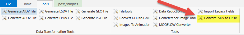
Disadvantages
- Files tend to be larger since a single screen can represent many points
- Displaying boring based data is more limited
- LPDV files cannot be further refined.
- If your points are too coarse or too fine, you cannot easily change this.
An explanation of the file format follows:
You may insert comment lines in .lpdv files.
- Comment lines must begin with a ’#’ as the first character of a line.
Entries on lines can be separated by commas, spaces and/or tabs.
The First (uncommented) line:
- Must begin with Elevation or Depth
- For the data section shown below, when Depth is specified, replace Z with Depth and columns 5 & 6 are required
- Then each material specified in the file is listed as: “Material^number^|Material^name^”
- The end of the line has the coordinate units (typically m [meters] or ft [feet]), OR the REPROJECT tag.
- Must begin with Elevation or Depth
The next line begins the data section. You do not need to specify the number of data lines. The 9 entries in each line are all requiredand therefore must be:
- Columns 1-3: X, Y, Z
- Column 4: Material-number (these are integers which should begin with zero on line 1)
- Column 5: Boring ID : OPTIONAL, however, if any line has this then all lines must have it.
- Column 6: Ground Surface Elevation: OPTIONAL, however, it can only be included if Boring_ID is included and if any line has this then all lines must have it.
Below is a snippet of the file “lithology.lpdv” in the “Exporting Data to C Tech File Formats” folder of Studio Projects. This file was converted from lithology.lsdv.
Elevation “0|SAND” “1|SANDSTONE” “2|GRAVEL” “3|MUDSTONE” “4|LIMESTONE” “5|SILTSTONE” “6|MADEGROUND” “7|CONGLOMERATE” “8|GYPSUM” “9|CLAY” “10|SILT” m
736133.267249 1637594.558440 1190.194000 0 720B0001 1190.200000
736133.267249 1637594.558440 1189.806000 0 720B0001 1190.200000
736133.267249 1637594.558440 1189.794000 1 720B0001 1190.200000
736133.267249 1637594.558440 1189.006000 1 720B0001 1190.200000
736133.267249 1637594.558440 1188.206000 1 720B0001 1190.200000
736133.267249 1637594.558440 1188.194000 0 720B0001 1190.200000
736133.267249 1637594.558440 1187.806000 0 720B0001 1190.200000
736133.267249 1637594.558440 1187.794000 1 720B0001 1190.200000
736133.267249 1637594.558440 1187.256000 1 720B0001 1190.200000
736133.267249 1637594.558440 1186.706000 1 720B0001 1190.200000
736133.267249 1637594.558440 1186.694000 0 720B0001 1190.200000
736133.267249 1637594.558440 1186.156000 0 720B0001 1190.200000
736133.267249 1637594.558440 1185.606000 0 720B0001 1190.200000
736133.267249 1637594.558440 1185.594000 2 720B0001 1190.200000
736133.267249 1637594.558440 1184.906000 2 720B0001 1190.200000
736133.267249 1637594.558440 1184.206000 2 720B0001 1190.200000
736133.267249 1637594.558440 1184.194000 1 720B0001 1190.200000
736133.267249 1637594.558440 1183.453000 1 720B0001 1190.200000
736133.267249 1637594.558440 1182.706000 1 720B0001 1190.200000
736133.267249 1637594.558440 1181.959000 1 720B0001 1190.200000
736133.267249 1637594.558440 1181.206000 1 720B0001 1190.200000
736133.267249 1637594.558440 1181.194000 1 720B0001 1190.200000
LSDV Lithology Screen Data Value File Format
The LSDV lithology file format can be used as a more feature rich replacement for the older PGF format. It has the following advantages:
- Fully supports non-vertical borings
- Supports missing intervals and lithology data which does not begin at ground surface
- Provides an Explicit definition of each lithologic interval
An explanation of the file format follows:
You may insert comment lines in .pgf files.
- Comment lines must begin with a ’#’ as the first character of a line.
Any line beginning with # is a comment (in the file below, the first and third lines are comments and could be deleted without loss of function)
Entries on lines can be separated by commas, spaces and/or tabs.
The First (uncommented) line:
- Must begin with Elevation or Depth
- For the data section shown below, when Depth is specified, replace Z with Depth
- Then each material specified in the file is listed as: “Material^number^|Material^name^”
- The end of the line has the coordinate units (typically m [meters] or ft [feet]), OR the REPROJECT tag.
- Must begin with Elevation or Depth
The next line begins the data section. You do not need to specify the number of data lines. The 9 entries in each line are all requiredand therefore must be:
- Columns 1-3: X, Y, Z
- Columns 4-6: X, Y, Z
- Column 7: Material-number (these are integers which should begin with zero on line 1)
- Column 8: Boring ID
- Column 9: Ground Surface Elevation
We cannot sort this data for you because some borings may turn to horizontal or even upwards.
- It is your responsibility to make sure that the data is in the proper order.
- It is your responsibility to make sure that each boring ID corresponds to a unique X, Y location if there would be overlapping Z (or depth) intervals. In other words, there cannot be overlapping boring definitions
Below is a snippet of the file “lithology.lsdv” in the “Exporting Data to C Tech File Formats” folder of Studio Projects.
C Tech Data Exporter generated LSDV File from LITHOLOGY-DATA.XLSX (05/01/2020 15:31:03)
Elevation “0|SAND” “1|SANDSTONE” “2|GRAVEL” “3|MUDSTONE” “4|LIMESTONE” “5|SILTSTONE” “6|MADEGROUND” “7|CONGLOMERATE” “8|GYPSUM” “9|CLAY” “10|SILT” m
Columns [DEMO]: “East” “North” “Elev-Top” “East” “North” “Elev-Bot” “Lithology” “Boring” “Ground_Surface”
736133.267249, 1637594.55844, 1190.2, 736133.267249, 1637594.55844, 1189.8, 0, “720B0001”, 1190.2
736133.267249, 1637594.55844, 1189.8, 736133.267249, 1637594.55844, 1188.2, 1, “720B0001”, 1190.2
736133.267249, 1637594.55844, 1188.2, 736133.267249, 1637594.55844, 1187.8, 0, “720B0001”, 1190.2
736133.267249, 1637594.55844, 1187.8, 736133.267249, 1637594.55844, 1186.7, 1, “720B0001”, 1190.2
736133.267249, 1637594.55844, 1186.7, 736133.267249, 1637594.55844, 1185.6, 0, “720B0001”, 1190.2
736133.267249, 1637594.55844, 1185.6, 736133.267249, 1637594.55844, 1184.2, 2, “720B0001”, 1190.2
736133.267249, 1637594.55844, 1184.2, 736133.267249, 1637594.55844, 1181.2, 1, “720B0001”, 1190.2
736133.267249, 1637594.55844, 1181.2, 736133.267249, 1637594.55844, 1176.2, 1, “720B0001”, 1190.2
736133.267249, 1637594.55844, 1176.2, 736133.267249, 1637594.55844, 1174.9, 1, “720B0001”, 1190.2
736286.268053, 1637647.55834, 1191.2, 736286.268053, 1637647.55834, 1190.2, 0, “720B0002”, 1191.2
736286.268053, 1637647.55834, 1190.2, 736286.268053, 1637647.55834, 1189.8, 0, “720B0002”, 1191.2
736286.268053, 1637647.55834, 1189.8, 736286.268053, 1637647.55834, 1187.2, 1, “720B0002”, 1191.2
736286.268053, 1637647.55834, 1187.2, 736286.268053, 1637647.55834, 1186.2, 2, “720B0002”, 1191.2
736286.268053, 1637647.55834, 1186.2, 736286.268053, 1637647.55834, 1184.1, 1, “720B0002”, 1191.2
736286.268053, 1637647.55834, 1184.1, 736286.268053, 1637647.55834, 1182.2, 1, “720B0002”, 1191.2
736286.268053, 1637647.55834, 1182.2, 736286.268053, 1637647.55834, 1175.9, 1, “720B0002”, 1191.2
737193.272266, 1637709.55665, 1190.2, 737193.272266, 1637709.55665, 1189.2, 0, “720B0003”, 1190.2
737193.272266, 1637709.55665, 1189.2, 737193.272266, 1637709.55665, 1188.2, 0, “720B0003”, 1190.2
737193.272266, 1637709.55665, 1188.2, 737193.272266, 1637709.55665, 1184.2, 0, “720B0003”, 1190.2
737193.272266, 1637709.55665, 1184.2, 737193.272266, 1637709.55665, 1181.9, 0, “720B0003”, 1190.2
737193.272266, 1637709.55665, 1181.9, 737193.272266, 1637709.55665, 1179.2, 1, “720B0003”, 1190.2
737193.272266, 1637709.55665, 1179.2, 737193.272266, 1637709.55665, 1178.9, 0, “720B0003”, 1190.2
737193.272266, 1637709.55665, 1178.9, 737193.272266, 1637709.55665, 1178.2, 1, “720B0003”, 1190.2
737193.272266, 1637709.55665, 1178.2, 737193.272266, 1637709.55665, 1177.9, 0, “720B0003”, 1190.2
737193.272266, 1637709.55665, 1177.9, 737193.272266, 1637709.55665, 1177.2, 1, “720B0003”, 1190.2
737193.272266, 1637709.55665, 1177.2, 737193.272266, 1637709.55665, 1174.7, 1, “720B0003”, 1190.2
GEO: Borehole Geology Stratigraphy
Geology data files basically contain horizontal and vertical coordinates, which describe the geometry of geologic features of the region being modeled. The files must be in ASCII format and can be delimited by commas, spaces, or tabs. Borehole Geology files must have a .geo suffix to be selected in the file browsers of EVS modules. The z values in .geo files can represent either elevation or depth, although elevation is generally the easiest to work with. When chemistry or property data is to be utilized along with geologic data for a 3-D visualization, a consistent coordinate system must be used in both sets of data.
Geology files should also specify the geologic layer material (color) number and layer names. This provides a mechanism to color multiple (not necessarily adjacent) layers as the same material.
Borehole Geology files (.geo suffix) must have the same number of entries for each boring location, so that every geologic layer in the system is represented in each boring. However, EVS allows flags to be included in the .geo files to allow automated processing of data in systems where geologic layers are not present in all locations (i.e., the layers “pinch out”). Also, EVS accommodates borings that were not extended deep enough to encounter layers that the scientist knows are present in the system. The use of these flags greatly facilitates the production of .geo data files, and minimizes the amount of manual interpretation the scientist must do before using EVS to analyze, understand, and refine a geologic model. For layers that pinch out, a flag of pinch can be used for automated estimation of the “depth” to the bottom of that layer. Entering this flag is essentially equivalent to entering the bottom depth of the layer directly above the pinched out layer (which is also an acceptable way to prepare the file). When EVS encounters this flag in a file, it assigns the pinched out layer a zero thickness at this location. For borings that do not extend to the depths of geologic layers in the system, a flag of short is included in the file for all layers below the depth of the boring. Including this flag notifies EVS to ignore the presence of this boring when kriging the surface of the layers below the total depth of the boring.
Format:
The file name must have a .geo suffix to be selected in the module’s file browser. The format below is the same for all EVS modules which read geology files:
You may insert comment lines in .geo files.
- Comment lines must begin with a ’#’ as the first character of a line.
The first non-commented line of the file is the header line (line 1 described below).
Line 1: Any header message: Except that:
- $W or $G as the first two characters signifies a special geology file which contains unrelated surfaces such as historical water tables. These flags turn off checking for corrupt geology file formats (situations where lower surfaces are above higher surfaces) and automatically turn off kriging in thickness space.
- Line one cannot be BLANK
Line 2: Elevation/Depth Specifier:
- The only REQUIRED item on this line in the Elevation or Depth Specifier.
- This line should contain the word Elevation or Depth (case insensitive) to denote whether sample elevations are true elevation or depth below ground surface.
- If set to Depth all surface descriptions for layer bottoms are entered as depths relative to the top surface. This is a common means of collecting sample coordinates for borings.
- Note that the flags such as pinch or short are not modified.
- This line should contain the word Elevation or Depth (case insensitive) to denote whether sample elevations are true elevation or depth below ground surface.
- Line 2 SHOULD contain names for each geologic surface (and therefore the layers created by them).
- There are some rules that must be observed.
- The number of surface (layer) names MUST be equal to the number of surfaces. Therefore, if naming layers, the first name should correspond to the top surface and each subsequent name will refer to the surface that defines the bottom of that layer.
- A name containing a space MUST be enclosed in quotation marks example (“Silty Sand”). Names should be limited to upper and lower case letters, numerals, hyphen “-” and underscore “_”. The names defined on line two will appear as the cell set name in the explode_and_scale or select cell sets modules. Names should be separated with spaces, commas or tabs.
- There are some rules that must be observed.
- Line 2: After the names, include the units of your coordinates (e.g. feet or meters). It must follow the names for each material number.
Line 3: The first integer (n) is the number of lines to follow. The second integer (m) is the number of geologic layer depths plus one (for the top surface). The 3rd and subsequent numbers are the colors for each surface in your model. Layers are colored by the color of the surface that defines their bottoms. The first two color numbers should be the same (top and bottom of the first layer).
When used with fence_geology, the order of the borings determines the connectivity of the fence diagram and must match the chemistry file for krig_fence.
Note that X and Y corresponding to Eastings and Northings are used. Be careful not to reverse these.
Line 4: First line of sample data. X, Y, top surface, and “m” depths or elevations to the bottom of each geologic layer. Coordinates, elevations (depths) and boring name can be separated by one comma and/or any number of spaces or tabs.
Two different flag parameters are included to accommodate special conditions. These flags are
A: Boring terminates early or surface information is missing. This flag class is used to identify that a boring did not continue deep enough to find the bottom of a geologic layer, OR that a section of a core sample is missing (lost, damaged, etc.) and that no determination of the location of this surface can be made from this boring. This is distinctly different than a surface (layer) that is not present because it has been determined that it has pinched out. The flags that are used for this class are [note: all flags are case insensitive, but spelling is critical]:
- missing
- unknown
- unk
- na
- short
- terminated
- term
In the sample file below, BOR-24 was not deep enough to reach to the bottom of the Lsand (lower sand) layer or the gravel layer. Rather than use the bottom of the boring (a meaningless number), the short flag is used so that this boring will not be used to determine the bottom of these two layers. Similarly BOR-72 is not deep enough to be used in determining the bottom of the last (Gravel) layer. The flags that are used for this class are [note: all flags are case insensitive, but spelling is critical]:
B: This flag class is used to identify that a geologic layer is not present because it has pinched out for this particular boring. It can be “thought of” as numerically equivalent to using the value one column to the left. However, now that gridding and horizons includes special treatment for the pinchflag, using the value to the left is not strictly equivalent.
- pinch
- pinched
- pinch-out
Note that several layers pinch out in borings WEL-67, BOR-23, BOR-70 and BOR-24, so the pinch flag was used for these layer’s entries instead of any numerical value.
IMPORTANT: There are two important things to consider when using the flags above:
- It is wholly inappropriate to have a pinch follow a short. Pinch denotes that the layer above is zero thickness. It is equivalent to using the numeric value to the left. However if it were to follow a short (unknown) it would be meaningless since the short is interpreted to be missing information.
- If your last defined surface has fewer than 3 numeric values (with all the rest being missing/short), it will be poorly defined since it takes 3 points to define a plane. If there are no numeric valuesthe surfacecannot be created.
…
Line 3+n is the last line of the file.
AN EXAMPLE FILE FOLLOWS:
| X | Y | TOP | BOT_1 | BOT_2 | BOT_3 | BOT_4 | BOT_5 | BOT_6 | BOT_7 | Boring |
|---|---|---|---|---|---|---|---|---|---|---|
| Depth | Top | Fill | SiltySand | Clay | Sand | Silt | Sand | Gravel | feet | |
| 7 | 8 | 5 | 5 | 3 | 1 | 4 | 2 | 4 | 6 | |
| 11856.7 | 12764.0 | 0 | 5.0 | 18.2 | 23.5 | pinch | pinch | 69.0 | 105.0 | WEL-67 |
| 11889.6 | 12772.2 | 0 | 1.5 | 17.0 | 22.0 | pinch | pinch | 63.0 | 105.0 | BOR-23 |
| 11939.1 | 12758.4 | 0 | 2.5 | 16.0 | 25.5 | pinch | pinch | 63.0 | 105.0 | BOR-70 |
| 12002.8 | 12759.8 | 0 | 1.0 | 17.0 | 27.0 | pinch | 47.0 | short | short | BOR-24 |
| 12085.1 | 12749.0 | 0 | 1.0 | 17.5 | 25.7 | 45.7 | pinch | 68.0 | 105.0 | WEL-71 |
| 12146.7 | 12713.2 | 0 | 1.0 | 18.0 | 26.5 | 32.5 | 39.5 | 65.0 | short | BOR-72 |
| 12199.7 | 12709.8 | 0 | 1.0 | 16.5 | 22.5 | 27.5 | 35.5 | 70.0 | 105.0 | WEL-12 |
This file has 7 boreholes with 8 entries (surfaces) per borehole, corresponding to the top surface and the bottom depths of 7 geologic layers. Note that the fourth and sixth layers are both designated to be material 4. This allows you to easily create layers with the same material the same color.
Other Examples of Geologic Input Files
Example of a .geo file for sedimentary layers and lenses (containing pinchouts)
Example of a .geo file for Dipping Strata Geologic_File_Example_Outcrop_of_Dipping_Strata
Geologic File Example: Sedimentary Layers and Lenses
Geologic File Example: Sedimentary Layers & Lenses Both example files below represent valid forms for the geology file associated with the above figure. For file 1, line 2 of the file is “1”, therefore all surface elevations are entered as actual elevations relative to a fixed reference such as sea level (not depths) and the relationship between x, y, and elevation must be a right handed coordinate system. Note that X and Y corresponding to Eastings and Northings are used. Be careful not to reverse these.
Geologic File Example: Outcrop of Dipping Strata
Geologic File Example: Outcrop of Dipping Strata EVS is not limited to sedimentary layers or lenses. The figure below shows a cross-section through an outcrop of dipping geologic strata. EVS easily model the layers truncating on the top ground surface. The file below represents the geology file associated with the above figure. Line 2 of the file is “Elevation”, therefore all surface elevations are entered as elevations (not depths) and the relationship between x, y, and elevation must be a right handed coordinate system. The pinch flag is used extensively to identify that a geologic layer is not present (pinched out) for a particular boring. It is equivalent to using the value one column to the left. The file was created with the assumption that there was no desire to model any layers below -70 foot elevation and that all borings extend to/beyond that depth.
Geology Files for Production of a Fence Diagram
Geology Files for Production of a Fence Diagram Discussion of Geology Files for Fence Sections Files used to create fence diagrams contain only those borings that the user wishes to include on an individual cross section of the fence, in the order that they will be connected along the section. The resulting set of files includes one .geo file for each cross section that will be included in a fence diagram. The order of the boring listings determines the connectivity of the fence diagram, and must match the order of the borings in the associated chemistry file when chemistry is to be displayed on the diagram. The data for the boring(s) at which individual sections will be joined to produce the fence diagram are included in each of the cross section files that will intersect. Generally, it is easiest to create the geology file for the complete 3-D dataset, and then cut and paste the individual section files from the complete file. Examples of a 3-D geology file and a typical set of fence diagram files are presented below.
Subsections of GEO: Borehole Geology Stratigraphy
Geologic File Example: Sedimentary Layers & Lenses
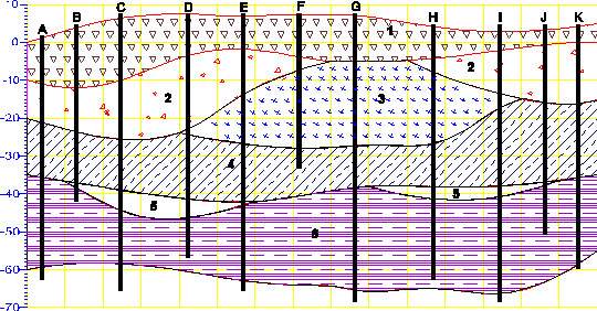
Both example files below represent valid forms for the geology file associated with the above figure. For file 1, line 2 of the file is “1”, therefore all surface elevations are entered as actual elevations relative to a fixed reference such as sea level (not depths) and the relationship between x, y, and elevation must be a right handed coordinate system. Note that X and Y corresponding to Eastings and Northings are used. Be careful not to reverse these.
Two special flags are used to accommodate special conditions. These flags are pinch and short. Pinch is used to identify that a geologic layer is not present (pinched out) for a particular boring. It is equivalent to using the value one column to the left. Short is used to identify that a boring did not extend to the bottom of a geologic layer. In the sample file below, boring C was not deep enough to reach to the bottom of the layer 3 or any subsequent layers. Rather than use the bottom of the boring (a meaningless number), the short flag is used so that this boring will not be used to determine the bottom of these layers.
File 1:
| X | Y | TOP | BOT_1 | BOT_2 | BOT_3 | BOT_4 | BOT_5 | BOT_6 | NAME |
|---|---|---|---|---|---|---|---|---|---|
| Elev | Top | FILL | SH | SS | SD | SLS | GR | feet | |
| 11 | 7 | 1 | 1 | 2 | 3 | 4 | 5 | 6 | |
| 5 | 3 | 3 | -11.5 | -22 | pinch | -36 | pinch | -59 | A |
| 13 | 5 | 3.5 | -12 | -22.5 | pinch | -36.8 | -37.5 | short | B |
| 24 | 7 | 5 | -11 | -24 | pinch | -38.5 | -43 | -58.6 | C |
| 42 | 2 | 8 | -3 | -22 | -23 | -41.5 | -46 | short | D |
| 57 | 11 | 7 | -2 | -13 | -26.5 | -42 | -43.5 | -63 | E |
| 72 | 14 | 7 | -3 | -8 | -27.6 | short | short | short | F |
| 85 | 19 | 5.7 | -5 | pinch | -26.6 | -38.3 | pinch | -65 | G |
| 107 | 23 | 4.2 | -5 | -8 | -26 | -38 | -41 | short | H |
| 123 | 35 | 2.2 | -3 | -13 | -16.9 | -37.5 | -41 | -66 | I |
| 136 | 24 | 3 | -1.5 | -15 | pinch | -37 | -37.5 | short | J |
| 145 | 18 | 4 | 0 | -15.7 | pinch | -36.3 | pinch | -58 | K |
For file 2 line 2 of the file is Depth", therefore all surface descriptions for layer bottoms are entered as depths relative to the top surface elevations. This is a common means of collecting sample coordinates for borings. Note that the flags (pinch and short) are not affected by using depths versus elevations.
File 2:
| X | Y | TOP | BOT_1 | BOT_2 | BOT_3 | BOT_4 | BOT_5 | BOT_6 | NAME |
|---|---|---|---|---|---|---|---|---|---|
| Depth | Top | FILL | SH | SS | SD | SLS | GR | feet | |
| 11 | 7 | 1 | 1 | 2 | 3 | 4 | 5 | 6 | |
| 5 | 3 | 3 | 14.5 | 25 | pinch | 39 | pinch | 62 | A |
| 13 | 5 | 3.5 | 15.5 | 26 | pinch | 40.3 | 41 | short | B |
| 24 | 7 | 5 | 16 | 29 | pinch | 43.5 | 48 | 63.6 | C |
| 42 | 2 | 8 | 11 | 30 | 31 | 49.5 | 54 | short | D |
| 57 | 11 | 7 | 9 | 20 | 33.5 | 49 | 50.5 | 70 | E |
| 72 | 14 | 7 | 10 | 15 | 34.6 | short | short | short | F |
| 85 | 19 | 5.7 | 10.7 | pinch | 32.3 | 44 | pinch | 70.7 | G |
| 107 | 23 | 4.2 | 9.2 | 12.2 | 30.2 | 42.2 | 45.2 | short | H |
| 123 | 35 | 2.2 | 5.2 | 15.2 | 19.1 | 39.7 | 43.2 | 68.2 | I |
| 136 | 24 | 3 | 4.5 | 18 | pinch | 40 | 40.5 | short | J |
| 145 | 18 | 4 | 4 | 19.7 | pinch | 40.3 | pinch | 62 | K |
There is no numerical equivalent to using the short flag. It causes the kriging modules to select only those borings with valid data for computing the surfaces of each layer.
Geologic File Example: Outcrop of Dipping Strata
EVS is not limited to sedimentary layers or lenses. The figure below shows a cross-section through an outcrop of dipping geologic strata. EVS easily model the layers truncating on the top ground surface.
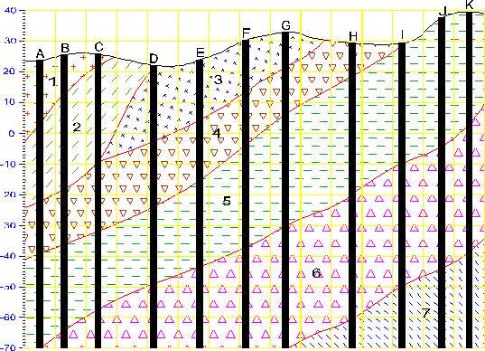
The file below represents the geology file associated with the above figure. Line 2 of the file is “Elevation”, therefore all surface elevations are entered as elevations (not depths) and the relationship between x, y, and elevation must be a right handed coordinate system. The pinch flag is used extensively to identify that a geologic layer is not present (pinched out) for a particular boring. It is equivalent to using the value one column to the left. The file was created with the assumption that there was no desire to model any layers below -70 foot elevation and that all borings extend to/beyond that depth.
Also, we have assigned the following material layer colors (numbers) to the 7 layers.
Layer # Material Abbreviation Material Color
1 Shale SH 5
2 Silty-sand SS 2
3 Sand SD 1
4 Sandy-silt SLS 3
5 Silty-sand SS 2
6 Sandy-silt SLS 3
7 Silt SL 4
| X | Y | TOP | BOT_1 | BOT_2 | BOT_3 | BOT_4 | BOT_5 | BOT_6 | BOT_7 | NAME |
|---|---|---|---|---|---|---|---|---|---|---|
| Elevation | Top | SH | SH | SS | SD | SLS | SS | SLS | SL | feet |
| 44 | 8 | 5 | 5 | 2 | 1 | 3 | 2 | 3 | 4 | |
| 5 | 3 | 23.5 | 4 | -22 | pinch | -39 | -70 | -70 | -70 | A |
| 13 | 5 | 26 | 13 | -18 | pinch | -36 | -64 | -70 | -70 | B |
| 24 | 7 | 26 | 22 | -9 | -9.5 | -32 | -57.5 | -70 | -70 | C |
| 42 | 2 | 22 | pinch | pinch | -3 | -24 | -50 | -70 | -70 | D |
| 57 | 6 | 24 | pinch | pinch | 4 | -15 | -43.5 | -70 | -70 | E |
| 72 | 7 | 30.5 | pinch | pinch | 14 | -4 | -37 | -70 | -70 | F |
| 85 | 3 | 33 | pinch | pinch | 21.5 | 6 | -30 | -70 | -70 | G |
| 107 | 4 | 29.5 | pinch | pinch | pinch | 19 | -20 | -60 | -70 | H |
| 123 | 6 | 29.5 | pinch | pinch | pinch | 28.5 | -10 | -49.5 | -70 | I |
| 136 | 3 | 38 | pinch | pinch | pinch | pinch | -4 | -44 | -70 | J |
| 145 | 0 | 39.5 | pinch | pinch | pinch | pinch | -3 | -39 | -70 | K |
| 3.11 | 28.18 | 25.93 | 3.96 | -20.99 | pinch | -39.01 | -70 | -70 | -70 | A1 |
| 16.85 | 37.97 | 24.85 | 15.61 | -20.7 | pinch | -35.7 | -61.92 | -70 | -70 | B1 |
| 25.99 | 32.02 | 23.05 | 23.34 | -6.11 | -6.41 | -31.53 | -59.17 | -70 | -70 | C1 |
| 41.05 | 25.13 | 24.26 | pinch | pinch | -1.22 | -25.57 | -47.06 | -70 | -70 | D1 |
| 54.43 | 34.94 | 26.56 | pinch | pinch | 1.36 | -14.66 | -45.49 | -70 | -70 | E1 |
| 67.29 | 29.3 | 28.3 | pinch | pinch | 16.45 | -6.49 | -37.22 | -70 | -70 | F1 |
| 88.89 | 25.31 | 32.92 | pinch | pinch | 19.17 | 6.16 | -27.28 | -70 | -70 | G1 |
| 104.17 | 30.58 | 30.13 | pinch | pinch | pinch | 19.76 | -22.25 | -62.18 | -70 | H1 |
| 121.87 | 30.26 | 30.76 | pinch | pinch | pinch | 27.84 | -7.81 | -49.67 | -70 | I1 |
| 136.99 | 29.61 | 35.95 | pinch | pinch | pinch | pinch | -6.02 | -44.8 | -70 | J1 |
| 149.67 | 29.33 | 37.59 | pinch | pinch | pinch | pinch | -4.09 | -40.17 | -70 | K1 |
| 4.06 | 62.03 | 23.47 | 3.46 | -22.43 | pinch | -38.05 | -70 | -70 | -70 | A2 |
| 12.09 | 64.15 | 25.26 | 13.42 | -19.11 | pinch | -33.89 | -59.06 | -70 | -70 | B2 |
| 30.73 | 66.42 | 25.81 | 26.1 | -3.46 | -3.76 | -28.81 | -58.62 | -70 | -70 | C2 |
| 40.43 | 49.79 | 26.12 | pinch | pinch | -0.5 | -27.73 | -46.67 | -70 | -70 | D2 |
| 54.5 | 65.51 | 27.88 | pinch | pinch | 1.79 | -15.51 | -43.8 | -70 | -70 | E2 |
| 66.41 | 52.9 | 25.48 | pinch | pinch | 16.96 | -7.18 | -35.22 | -70 | -70 | F2 |
| 93.58 | 50.18 | 34.29 | pinch | pinch | 21.62 | 6.46 | -28.76 | -70 | -70 | G2 |
| 106.13 | 55.44 | 30.39 | pinch | pinch | pinch | 20.9 | -23.47 | -60.65 | -70 | H2 |
| 126.19 | 63.43 | 28.78 | pinch | pinch | pinch | 27.64 | -8.31 | -48.85 | -70 | I2 |
| 138.39 | 62.4 | 36.52 | pinch | pinch | pinch | pinch | -5.72 | -47.12 | -70 | J2 |
| 144.91 | 52.79 | 40.49 | pinch | pinch | pinch | pinch | -4.66 | -37.23 | -70 | K2 |
| 6.77 | 86.15 | 21.09 | 2.83 | -22.62 | pinch | -36.05 | -70 | -70 | -70 | A3 |
| 16.91 | 98.53 | 22.86 | 10.95 | -17.19 | pinch | -31.33 | -57.46 | -70 | -70 | B3 |
| 35.07 | 87.05 | 25.39 | 25.81 | -2.37 | -2.67 | -30.89 | -59.85 | -70 | -70 | C3 |
| 36.37 | 77.38 | 26.62 | pinch | pinch | -2.19 | -27.56 | -43.87 | -70 | -70 | D3 |
| 51.5 | 94.86 | 27.26 | pinch | pinch | 4.57 | -15.51 | -46.35 | -70 | -70 | E3 |
| 71.23 | 73.19 | 26.45 | pinch | pinch | 16.19 | -9.22 | -38.04 | -70 | -70 | F3 |
| 93.09 | 79.15 | 33.93 | pinch | pinch | 19.64 | 9.37 | -28.16 | -70 | -70 | G3 |
| 110.18 | 76.02 | 27.4 | pinch | pinch | pinch | 20.63 | -21.81 | -63.39 | -70 | H3 |
| 127.9 | 90.62 | 31.64 | pinch | pinch | pinch | 29.56 | -8.26 | -45.96 | -70 | I3 |
| 139.27 | 96.26 | 37.57 | pinch | pinch | pinch | pinch | -8.29 | -47.67 | -70 | J3 |
| 143.52 | 75.62 | 38.22 | pinch | pinch | pinch | pinch | -6.59 | -37.51 | -70 | K3 |
Geology Files for Production of a Fence Diagram
Discussion of Geology Files for Fence Sections
Files used to create fence diagrams contain only those borings that the user wishes to include on an individual cross section of the fence, in the order that they will be connected along the section. The resulting set of files includes one .geo file for each cross section that will be included in a fence diagram. The order of the boring listings determines the connectivity of the fence diagram, and must match the order of the borings in the associated chemistry file when chemistry is to be displayed on the diagram. The data for the boring(s) at which individual sections will be joined to produce the fence diagram are included in each of the cross section files that will intersect. Generally, it is easiest to create the geology file for the complete 3-D dataset, and then cut and paste the individual section files from the complete file. Examples of a 3-D geology file and a typical set of fence diagram files are presented below.
The format of the data in the file is exactly the same as for 3-D geology files. Material colors are not supported for fence diagrams.
An example set of files for producing a fence diagram with two merged cross sections are shown below:
| Geology File for Cross Section A-A' | ||||||
|---|---|---|---|---|---|---|
| Elevation | feet | |||||
| 7 | 8 | |||||
| 11086.52 | 12830.67 | 2500 | 2496 | 2484 | 2479 | 2420 |
| 11199.04 | 12810.16 | 2501 | 2492 | 2482 | 2473 | 2420 |
| 11259.67 | 12819.29 | 2502 | 2492 | 2479 | 2467 | 2425 |
| 11298 | 12808.63 | 2503 | 2492 | 2492 | 2480 | 2424 |
| 11414.4 | 12781.1 | 2504 | 2491 | 2482 | 2471 | 2420 |
| 11427 | 12780.9 | 2501 | 2493 | 2477 | 2467 | 2424 |
| 11496.34 | 12753.59 | 2502 | 2492 | 2480 | 2465 | 2422 |
| Geology File for Cross Section B B' | ||||
|---|---|---|---|---|
| Elevation | feet | |||
| 5 | 8 | |||
| 11209.35 | 12993.94 | 2502 | 2492 | 2481 |
| 11251.30 | 12929.27 | 2503 | 2493 | 2474 |
| 11248.75 | 12870.91 | 2501 | 2492 | 2483 |
| 11199.04 | 12810.16 | 2501 | 2492 | 2482 |
| 11211.87 | 12710.75 | 2503 | 2493 | 2480 |
This example fence diagram contains two cross sections, with elevations for the surface and the bottoms of seven layers of geology in each. Section A-A’ has seven borings that will be used to define it, and Section B-B’ has five borings. Neither of the sections contains layers that pinch out, and all of the borings extend to the depth of the fence. Note that the entries for location BOR-51 are identical in each file, and are placed such that the sections will cross at the second location in the A-A’ file, and the fourth location in the B-B’ file. The user will typically use a basemap to plan the orientations and intersections of the fences. EVS does not impose any restrictions on the number of borings in or placement of sections in fence diagrams, but planning should be done to assure that most sections of the fence can be viewed from a chosen viewpoint.
Geology Multi-File
Geology Multi-Files: Unlike the .geo file format, the .gmf format is not based on boring observations with common x,y coordinates. The multi-file format allows for description of individual geologic surfaces by defining a set of x,y,z coordinates (separated by spaces, tabs, and/or commas). Geologic hierarchy still applies for definition of complex geologic structures.
This file format allows for creation of geologic models when the data available for the top surface and one or more of the subsurface layers are uncorrelated (in number or x,y location). For example, a gmf file may contain 1000 x,y,z measurements for the ground surface, but only 12 x,y,z measurements for other lithologic surfaces. This format also allows for specification of the geologic material color (layer material number).
You SHOULD include the units of your coordinates (e.g. feet or meters). If this is included it must be on a line following the word units.
Note: there are no special flags (e.g. short, pinch, etc.) used in GMF files. Since each surface stands on its own (does not refer to a prior surface) pinched-out layers are accomplished by duplicating the elevations (x,y,z points) on two consecutive surfaces. The “short” flags are not needed since those points are merely excluded from a surface’s definition.
The name for a surface can be a date or date & time if the data represents surface points at different times (e.g. changing groundwater elevations. The date format is dependent on your REGIONAL SETTINGS on your computer (control panel).
C Tech uses the SHORT DATE and SHORT TIME formats.
If the date/time works in Excel it will likely work in EVS.
For most people in the U.S., this would not be 24 hour clock so you would need:
“m/d/yyyy hh:mm:ss AM” or “m/d/yyyy hh:mm:ss PM”
Also, you MUST put the date/time in quotes if you use more than just date (i.e. if there are spaces in the total date/time).
Format: The following is a geology multi-file which is included with EVS. This file begins with the line starting with a “#”.
Lines beginning with a “#” character are comments.
Each geologic surface begins with a line: surface x
The number after surface is the layer material color number.
Each surface can have different x,y coords and number of points
units ft
surface 2 Top
11086.5 12830.7 4.5
11199.0 12810.2 4
Comment lines can be placed anywhere in a multi-file
11259.7 12819.3 2
11298.0 12808.6 3
11414.4 12781.1 2
11427.0 12780.9 6.5
11496.3 12753.6 1.5
11209.4 12993.9 2
11251.3 12929.3 2
11248.8 12870.9 3
11211.9 12710.8 2
11302.0 13079.7 4.5
11286.8 13026.7 2
11309.0 12949.0 4
11340.5 12892.6 2.5
11338.0 12830.8 4
11393.5 12948.9 3.5
11401.7 12897.8 4
11416.9 12819.5 2.5
11381.7 12747.5 1.5
11410.3 12724.7 0.5
11566.3 12850.6 2.5
11586.3 13050.6 11.5
11086.3 13090.6 8.5
surface 2 Fill
11086.5 12830.7 -3.8
11199.0 12810.2 -5
11259.7 12819.3 -7.5
11298.0 12808.6 -6
11414.4 12781.1 -6
11427.0 12780.9 -7
11496.3 12753.6 -7.5
11209.4 12993.9 -3
11251.3 12929.3 -2.5
11248.8 12870.9 -3.5
11211.9 12710.8 -6.5
11302.0 13079.7 -3.5
11286.8 13026.7 -5
11309.0 12949.0 -2.5
11340.5 12892.6 -2.5
11338.0 12830.8 -8.8
11393.5 12948.9 -3.8
11401.7 12897.8 -2
11416.9 12819.5 -5
11381.7 12747.5 -4
11410.3 12724.7 -4.5
11566.3 12850.6 -5
11586.3 13050.6 1
11086.3 13090.6 -1
surface 1 Silt
11086.5 12830.7 -21
11199.0 12810.2 -20
11259.7 12819.3 -20.5
11298.0 12808.6 -19
11414.4 12781.1 -20.5
11427.0 12780.9 -23
11496.3 12753.6 -20
11209.4 12993.9 -23
11251.3 12929.3 -22
11248.8 12870.9 -22
11211.9 12710.8 -22.5
11302.0 13079.7 -21.9
11286.8 13026.7 -23
11309.0 12949.0 -22
11340.5 12892.6 -20
11338.0 12830.8 -23
11393.5 12948.9 -23
11401.7 12897.8 -22
11416.9 12819.5 -21
11381.7 12747.5 -21.5
11410.3 12724.7 -22.9
11566.3 12850.6 -21
11586.3 13050.6 -11
11086.3 13090.6 -14
surface 3 Clay
11086.5 12830.7 -26
11199.0 12810.2 -25
11259.7 12819.3 -27
11298.0 12808.6 -25.8
11414.4 12781.1 -28
11427.0 12780.9 -28.5
11496.3 12753.6 -28.8
11209.4 12993.9 -27.5
11251.3 12929.3 -28
11248.8 12870.9 -28.5
11211.9 12710.8 -27.5
11302.0 13079.7 -26
11286.8 13026.7 -29
11309.0 12949.0 -28.3
11340.5 12892.6 -23
11338.0 12830.8 -26.5
11393.5 12948.9 -27
11401.7 12897.8 -27.5
11416.9 12819.5 -28.5
11381.7 12747.5 -25.8
11410.3 12724.7 -25
11566.3 12850.6 -28.5
11586.3 13050.6 -18.5
11086.3 13090.6 -23.5
surface 5 Gravel
11086.5 12830.7 -42
11199.0 12810.2 -39
11259.7 12819.3 -40
11298.0 12808.6 -41.8
11414.4 12781.1 -42
11427.0 12780.9 -38.5
11496.3 12753.6 -38.8
11209.4 12993.9 -37.5
11251.3 12929.3 -40
11248.8 12870.9 -36.3
11211.9 12710.8 -37.5
11302.0 13079.7 -38
11286.8 13026.7 -37
11309.0 12949.0 -38.3
11340.5 12892.6 -38
11338.0 12830.8 -36.5
11393.5 12948.9 -39
11401.7 12897.8 -37.5
11416.9 12819.5 -38.5
11381.7 12747.5 -42.8
11410.3 12724.7 -36
11566.3 12850.6 -38.5
11586.3 13050.6 -26.5
11086.3 13090.6 -32.5
surface 4 Sand
11086.5 12830.7 -55
11199.0 12810.2 -53
11259.7 12819.3 -53
11298.0 12808.6 -55
11414.4 12781.1 -55
11427.0 12780.9 -51
11496.3 12753.6 -51
11209.4 12993.9 -51
11251.3 12929.3 -53
11248.8 12870.9 -50
11211.9 12710.8 -51
11302.0 13079.7 -51
11286.8 13026.7 -50
11309.0 12949.0 -52
11340.5 12892.6 -52
11338.0 12830.8 -50
11393.5 12948.9 -52
11401.7 12897.8 -51
11416.9 12819.5 -51
11381.7 12747.5 -56
11410.3 12724.7 -49
11566.3 12850.6 -51
11586.3 13050.6 -47
11086.3 13090.6 -48
end
ctech_example.gmf Database Generated GMF File (Creation at 7/22/2003 5:36:07 PM) Surface 1: 25 Coordinates Database Columns [GMF_Surface0 (Ground Surface)]: X, Y, Top surface 1 Sand
Subsections of Geology Multi-File
ctech_example.gmf
Database Generated GMF File (Creation at 7/22/2003 5:36:07 PM)
Surface 1: 25 Coordinates
Database Columns [GMF_Surface0 (Ground Surface)]: X, Y, Top
surface 1 Sand
11566.34 12850.59 2.5
11586.34 13050.59 11.5
11086.3 13090.6 8.5
.
.
.
.
11393.47 12948.9 3.5
11251.3 12929.27 2
Surface 1 Complete
Surface 2: 24 Coordinates (Added at 7/22/2003 5:37:04 PM)
Database Columns [GMF_Surface1]: X, Y, Z
surface 1 Sand
11566.34 12850.59 -5
11586.34 13050.59 1
11086.3 13090.6 -1
.
.
.
.
11393.47 12948.9 -3.8
11251.3 12929.27 -2.5
Surface 2 Complete
Surface 3: 24 Coordinates (Added at 7/22/2003 5:38:18 PM)
Database Columns [GMF_Surface2]: X, Y, Z
surface 1 Sand
11566.34 12850.59 -21
11586.34 13050.59 -11
11086.3 13090.6 -14
.
.
.
11393.47 12948.9 -23
11251.3 12929.27 -22
Surface 3 Complete
units ft
end
Database Generated GMF File (Finalization at 7/22/2003 5:39:06 PM)
.PT File Format
The .PT (Place-Text) format is used to place 3D text (labels) with user adjustable font and alignment.
The format is:
Lines beginning with “#” are comments
Lines beginning with “LINEFONT” are font specification lines specifically associated with single line text.
- LINEFONT, height, justification, azimuth, inclination, roll, red, green, blue, curve tolerance, font flags (bold is ignored)
- NOTE: There is no specification of the Font to be used, because EVS includes its own Unicode Line Font which supports most worldwide languages.
Lines beginning with “TRUETYPE” are font specification lines specifically associated with TrueType Fonts.
- TRUETYPE, height, justification, azimuth, inclination, roll, red, green, blue, curve tolerance, outlined (“True”/“False”), depth, bevel, font flags, font name
Lines beginning with “FORWARDFACING” font specification lines specifically associated with Forward Facing Fonts.
- FORWARDFACING, red, green, blue, font flags
- NOTE: Forward Facing font specifications other than color are module wide. Therefore, the .PT files do not contain the Justification or Font specification options (including size).
The lines containing each TEXT STRING to be displayed have five columns of information:
- X coordinate
- Y coordinate
- Z coordinate
- Explode_ID: This is equivalent to the (Stratigraphic) cell data “Layer” information. The uppermost ID (layer) is ZERO (0) and does not move. If you don’t want your text to move with changing Explode Distance, use a value of ZERO. Otherwise, by assigning an appropriate ID value your text string can move properly with both stratigraphic layers or lithologic materials as they are exploded.
- Text: Everything on the line after Explode_ID (and any trailing spaces) is the text to be placed at the above coordinate, and must be in quotes.
Blank lines anywhere in the file are ignored.
Lines beginning with “END” specify the end of the file. Using END is optional, but if you want to have any notes or comments after the last command or data line, precede it with a line using the “END” statement.
Lines beginning with “FONT” are legacy font specification lines that we suggest you avoid. However, when we read a legacy file, we attempt to migrate it to the new options.
Below is an example .PT file and the output it creates:
TRUETYPE, 20.000000, LC, 180.000000, 90.000000, 0.000000, 0.847059, 0.847059, 0.858824, 0.050000, False, 0.200000, 5.000000, None, “Noto Sans”
0.000000, 300.000000, 0.000000, 0, “TTF”
TRUETYPE, 20.000000, LC, 180.000000, 90.000000, 0.000000, 0.847059, 0.847059, 0.858824, 0.050000, False, 0.200000, 5.000000, Bold, “Noto Sans”
250.000000, 300.000000, 0.000000, 0, “TTF Bold”
TRUETYPE, 20.000000, LC, 180.000000, 90.000000, 0.000000, 0.847059, 0.847059, 0.858824, 0.050000, False, 0.200000, 5.000000, Italic, “Noto Sans”
500.000000, 300.000000, 0.000000, 0, “TTF Italic”
TRUETYPE, 20.000000, LC, 180.000000, 90.000000, 0.000000, 0.847059, 0.847059, 0.858824, 0.050000, False, 0.200000, 5.000000, Bold Italic, “Noto Sans”
750.000000, 300.000000, 0.000000, 0, “TTF Bold Italic”
TRUETYPE, 20.000000, UC, 180.000000, 90.000000, 0.000000, 0.847059, 0.847059, 0.858824, 0.050000, True, 0.200000, 5.000000, None, “Noto Sans”
0.000000, 200.000000, 0.000000, 0, “Outlined”
TRUETYPE, 20.000000, UC, 180.000000, 90.000000, 0.000000, 0.847059, 0.847059, 0.858824, 0.050000, True, 0.200000, 5.000000, Bold, “Noto Sans”
250.000000, 200.000000, 0.000000, 0, “Outlined Bold”
TRUETYPE, 20.000000, UC, 180.000000, 90.000000, 0.000000, 0.847059, 0.847059, 0.858824, 0.050000, True, 0.200000, 5.000000, Italic, “Noto Sans”
500.000000, 200.000000, 0.000000, 0, “Outlined Italic”
TRUETYPE, 20.000000, UC, 180.000000, 90.000000, 0.000000, 0.847059, 0.847059, 0.858824, 0.050000, True, 0.200000, 5.000000, Bold Italic, “Noto Sans”
750.000000, 200.000000, 0.000000, 0, “Outlined Bold Italic”
TRUETYPE, 20.000000, UC, 180.000000, 90.000000, 45.000000, 0.847059, 0.847059, 0.858824, 0.050000, False, 0.200000, 5.000000, Bold, “Noto Sans”
250.000000, 400.000000, 0.000000, 0, “TTF Bold at 45° roll”
LINEFONT, 20.000000, UC, 180.000000, 90.000000, 0.000000, 0.847059, 0.847059, 0.858824, 0.050000, None
0.000000, 100.000000, 0.000000, 0, “Singleline”
LINEFONT, 20.000000, UC, 180.000000, 90.000000, 0.000000, 0.847059, 0.847059, 0.858824, 0.050000, Italic
500.000000, 100.000000, 0.000000, 0, “Singleline Italic”
FORWARDFACING, 0.847059, 0.847059, 0.858824, None
0.000000, 0.000000, 0.000000, 0, “ForwardFacing”
This legacy format has been deprecated and replaced by the .PT File Format.
The EMT (EVS Multi-Text) format is used to place 3D text (labels) with user adjustable font and alignment.
The format is:
- Lines beginning with “#” are comments
- Lines beginning with “FONT” are font specification lines (more later)
- Lines beginning with “END” specify the end of the file (this is optional, but if you want to have anything after the last command or data line, precede it with an “END” statement.
- All other lines are DATA lines specifying the x-y-z coordinates of a string and the text for that string.
- Blank lines are ignored.
- The FONT specification lines contain the following information in this order:
- Size: The font size is the height of a typical Capitol letter in true user units
- Justification: The justification options are the same as in post_samples
- Plane: The plane options are the same as in post_samples
- Orientation: The orientation options are the same as in post_samples
- Red, Green, Blue: These 3 numbers determine the font color.
- Resolution: The resolution parameter is the same as in post_samples
- Depth: The parameter is the same as in post_samples
- Bevel%: The Bevel percentage isthe same as in post_samples
- Font Face: The Font Face options are the same as in post_samples
- Size: The font size is the height of a typical Capitol letter in true user units
- The DATA lines contain four columns of information:
- X coordinate
- Y coordinate
- Z coordinate
- Text: Everything on the line after the z coordinate (and trailing spaces) is the text to be placed at the above coordinate.
Below is an example EMT File
FONT Size Just. Plane Orient R G B Resolution Depth Bevel% Font Face
FONT, 4, MC, XZ, +X, 0.8, 0.8, 0.8, 3, 0, 0, Arial
X, Y, Z, Bore
11566.34, 12850.59, 8.5, B-30
11586.34, 13050.59, 12.5, B-31
11381.7, 12747.5, 2.5, B-33
11414.4, 12781.1, 3, B-34
11410.29, 12724.69, 4.5, B-4
11427, 12780.9, 7.5, B-42
11086.52, 12830.67, 5.5, B-49
11211.87, 12710.75, 3, B-50
11199.04, 12810.16, 5, B-51
11496.34, 12753.59, 2.5, B-53
11209.35, 12993.94, 3, B-57
11301.97, 13079.66, 5.5, B-58
11286.77, 13026.7, 3, B-59
FONT Size Just. Plane Orient R G B Resolution Depth Bevel% Font Face
FONT, 6, MC, XZ, +X, 1, 0.5, 0.5, 3, 0.1, 0, Arial
11393.47, 12948.9, 4.5, B-60
11309.03, 12948.99, 5, B-56
11248.75, 12870.91, 4, B-48
11259.67, 12819.29, 3, B-46
11298, 12808.63, 4, B-52
11338, 12830.8, 5, B-38
11401.73, 12897.77, 5, B-45
11416.9, 12819.45, 3.5, B-44
FONT, Size, Justification, Plane, Orientation, Red, Green, Blue, Resolution, Depth, Bevel%, Font Face
FONT, 8, MC, XZ, +X, 1, 0, 0, 3, .3, 0, Arial Bold
11340.49, 12892.61, 3.5, B-47
11251.3, 12929.27, 3, B-75
END