The collection and formatting of data for volumetric modeling is often the most challenging task for novice EVS users. This tutorial covers the instructions for preparing and reviewing all types of data commonly used in Earth Science modeling projects.

The next topics will demonstrate how to visualize these file formats, helping to ensure the quality and consistency of your data.

The following guidelines will simplify your data preparation:

• Use a single consistent coordinate projection (e.g. UTM, State Plane, etc.) for all data files used on a project, ensuring that X, Y and Z coordinate units are the same (e.g. meters or feet).
• For each file, you must know whether your Z coordinates represent Elevation or Depth below ground surface (most EVS data formats will accommodate both)
• Understand the data formats and what they represent. Below is a list of C Tech’s primary ASCII input file formats:
  • Geologic Data
    • PGF: A PGF file can be considered a group of file sections where each section represents the lithology for individual borings (wells). Typical borings logs can be easily converted to PGF format, and many boring log software programs export C Tech’s PGF format directly.
    • GEO: This file format represents a series of stratigraphic horizons which define geologic layers. GEO files are limited to data collected from vertical borings and require interpretation to handle pinched layers and dipping strata. The create stratigraphic hierarchy module may be used to create GEO files from PGF files, though they can be created in other ways.
    • GMF: This file format represents a series of stratigraphic horizons which define geologic layers. GMF files are not limited to vertical borings as GEO files are. Each horizon can have any number of X-Y-Z coordinates, however interpretation is still required to handle pinched layers and dipping strata. The create stratigraphic hierarchy module may be used to create GMF files from PGF files.
  • Analytical Data
    • Analytical Data files can be used for many types of data and industries including:
      • Chemical or assay measurements
      • Geophysical data (density, porosity, conductivity, gravity, temperature, seismic, resistance, etc.)
      • Oceanographic & Atmospheric data (conductivity, temperature, salinity, plankton density, etc.)
      • Time domain data representing any of the above analytes
    • APDV: The Analytical Point Data Values (.apdv) format should be used for all analytical data which is (effectively) measured at a point. Even data which is measured over small consistent (less than 1-2% of vertical model extent) intervals should normally be represented as being measured at a single point (X-Y-Z coordinate) at the midpoint of the interval. Time domain data for a single analyte should use this format.
    • AIDV: The Analytical Interval Data Values (.aidv) format should be used for all analytical data which is measured over a range of elevations (depths). Data which is measured over variable intervals, usually exceeding 2% of vertical model extent should use this format. Time domain data for a single analyte should use this format.
• The C Tech Data Exporter will export the above formats for data in Excel files and Microsoft Access databases. In all cases, the data source must contain sufficient information to create the desired output.

It is important to view your data prior to using it to build a model. There are many common file errors that can be quickly detected by viewing your raw data files, including:

• Transposing X & Y (Easting and Northing) coordinates
• Using Depth or Elevations incorrectly
• Consistency of geologic and analytical data

Let’s begin by creating a very simple application. In the Modules pane in the Application window, type p in the Search for Module section.

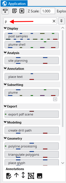
Notice that as soon as you type p, only those modules which start with this letter are displayed. The one we want in the first one listed, “post samples”.

We now want to copy the post_samples module into our Application window. We do this using the mouse. Left-click on “post samples” in the Modules window and hold the mouse down. Drag post samples to the Application Network window and place it above the viewer as shown below.

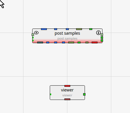
Note that post samples has a red border along the bottom. This tells us that the module has not yet run. This visual indication is very useful, especially with complex applications.

The next step is to connect post samples and the viewer. You can see that the only port color they have in common is red. Left-click in the red output port of post samples:

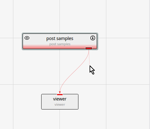
Then, while holding down the left-mouse, drag a short distance from the port, but near the thin-red connection, until the connection becomes bolder.

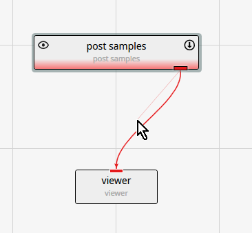
At this point, release the left mouse button and the connection is made. The reason for the thin and bolder lines is that there are often multiple modules that can be connected. All will be shown thin, but only the connection which is closest to the cursor will be bold.

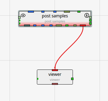
Deleting a connection

If we make an incorrect connection, we can delete the connection. To delete the connection, merely click on it to highlight it and then press the Delete key on your keyboard.

With the simple application from the previous topic, let’s read a PGF file and see that data represented in the viewer.

Double-left-click on post samples in the Application Network window to make its settings editable in the Properties window.

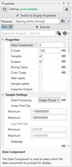
post samples will automatically adjust many of its settings based on the type of file read. Click on the Open button and browse to the Lithologic Geologic Modeling folder in Studio Projects and select dipping_strata_lens.pgf.

post samples will automatically run and your viewer should show a top view of:

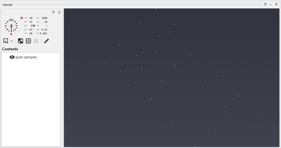
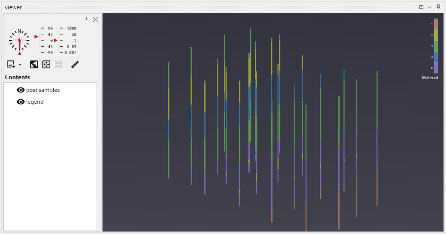
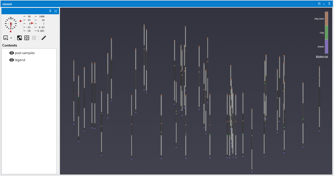
By default, we are seeing a top view of the borings represented in the PGF file. Using the left mouse button, rotate the view so you can see the 3D borings which are colored by lithology (geologic material).

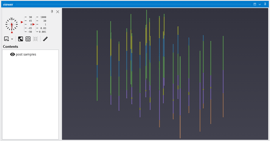
The image above demonstrates the default display of PGF (pregeology) files. The lithology intervals are colored by material and spheres are located at the beginning and end of each interval.

The colors represent material and range from purple (low) to orange-brown (high). Since this is geology, let’s add a legend to make it clear what materials correspond to our colors.

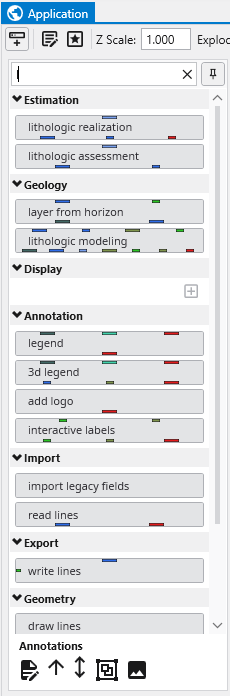
Type “l” in the Modules pane in the Application window and it will display

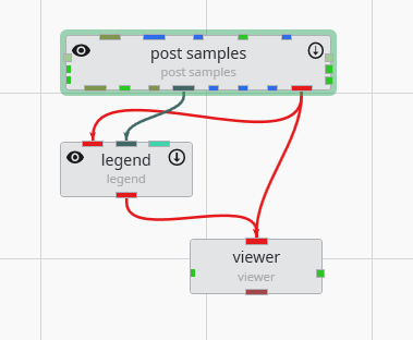
Copy legend to the Application (left-click and drag) and make the new connections as shown below

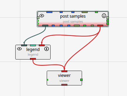
You can move the modules around so that your application and the associated connections between modules is as clear as possible. However, the arrangement (placement) of the modules does not affect how the application behaves. With legend our view becomes:

In the next topic, Viewing GEO Files, we’ll adjust colors

To view a GEO file, the process is nearly identical as with PGF.

Replace post_samples with a fresh instance of the module because when we read different file types, there are many settings in post samples which can change:

Click on the Open button and browse to the Lithologic Geologic Modeling folder in Studio Projects and select railyard_pgf.geo.

Your viewer (after rotating) should show:

Your first question might be, why are the borings so short?

Welcome to the real world. In the last topic we were dealing with a site where the z-extent was comparable to the x & y extents. But for this site, the z extent is 5-10% of the x-y extent. In order to better see the Stratigraphy represented by our .GEO file, we need to apply some vertical exaggeration, which we also refer to as Z-Scale.

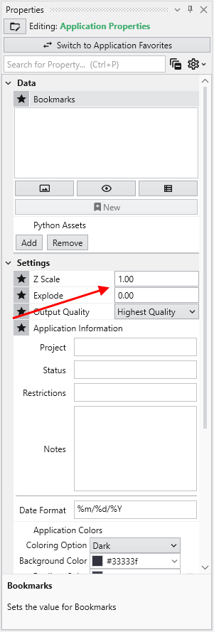
We find the Z-Scale parameter in one of 2 places. Either at the top of the Application window:

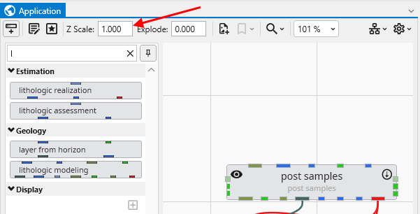
or in the Application Properties. To get to the Application Properties, double click on any blank space (not on a module or connection) in the Application.

Notice if we change it here, to be 5, it changes on the Home tab and in every module which has a Z-Scale. Our viewer now shows:

Please note: We could have changed the Z-Scale in post samples, but by doing so, we would have broken its link to the Global Z-Scale on the Home tab and Application Properties. In general you want all modules to share the Global Z-Scale, but there are times when you want control on a module-by-module basis. That is why we allow both.

GMF files are different than most other C Tech file formats in that the data is specifically NOT associated with borings. GMF files can be viewed using post samples, but file statistics can often be more useful, especially when dealing with large datasets.

Let’s build a new application:

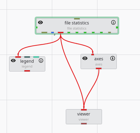
file statistics (and post samples) will only display a single surface of a GMF file at one time. The advantage of file statistics is that it will provide the extents and basic statistics information. The Data Component parameter determines which surface is displayed. 0 (zero) is the first surface.

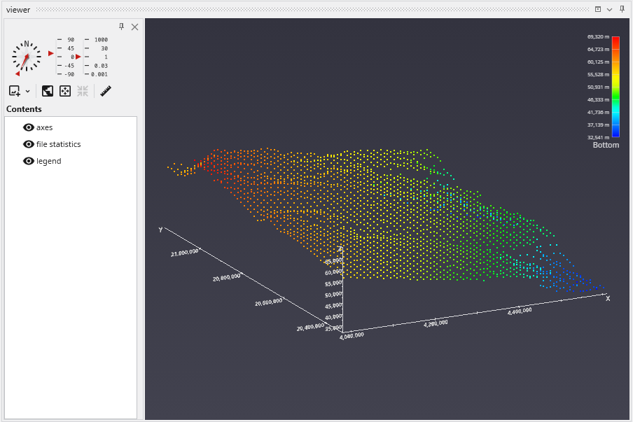
file statistics outputs points which are colored by elevation (for GMF files).

Double click on file statistics and select the file Reference\bottom.gmf. In the Application window at the top or the Application Properties, make sure the Z-Scale is set to 5.0.

The viewer should show:

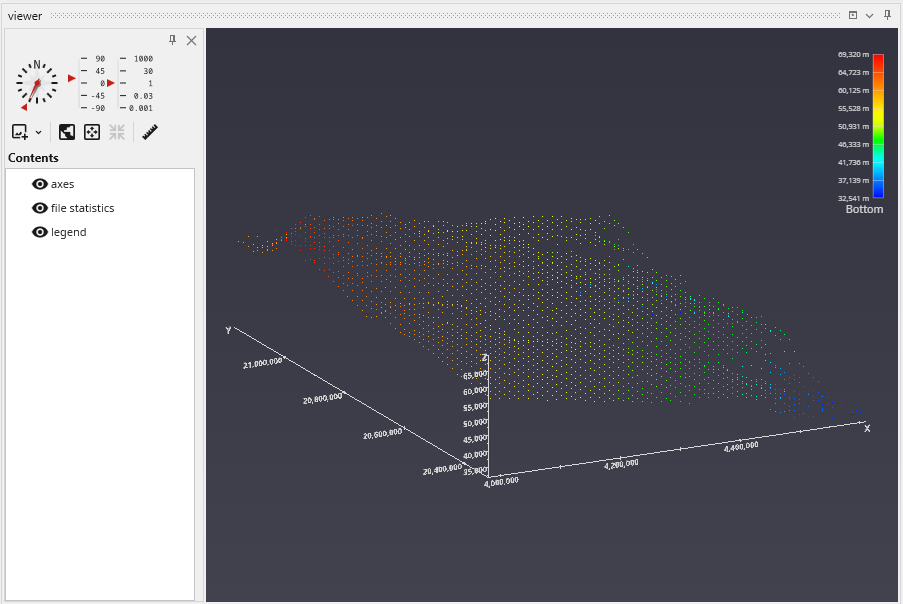
In the view above, each point is displayed as a single pixel point. You can increase the size to be a square of 2x2 pixels or larger using the Point Width parameter.

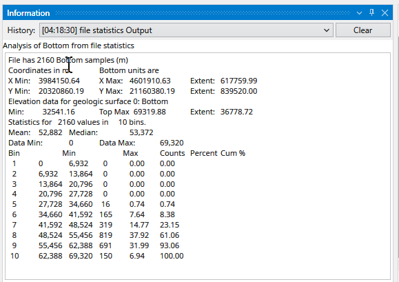
When file statistics runs, it provides the following information to the Information window.

Note that Number of Bins was set to 10, and Detailed Statistics was turned on.

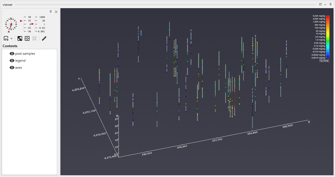
APDV files represent analyte data which is measured at points. The data can be collected at scattered locations or along borings. When boring IDs are included in the file, post samples will draw the borings as well as the samples.

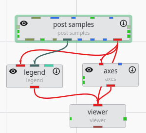
Create the following application. It is nearly identical to the application used for PGF files, but we do not need to connect the yellow port which contains geology or lithology names, as those are not applicable to APDV (or AIDV) files. However, if you do connect it, it won’t hurt anything.

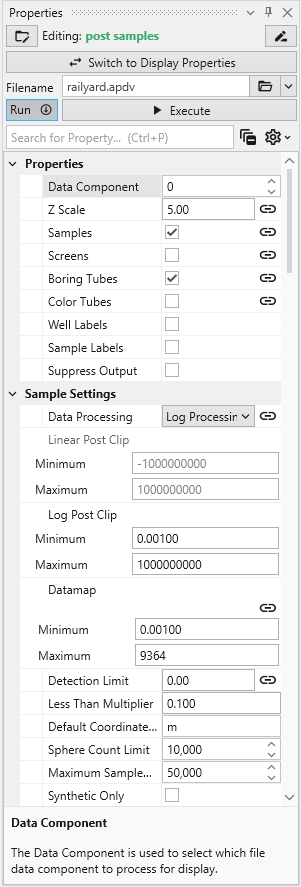
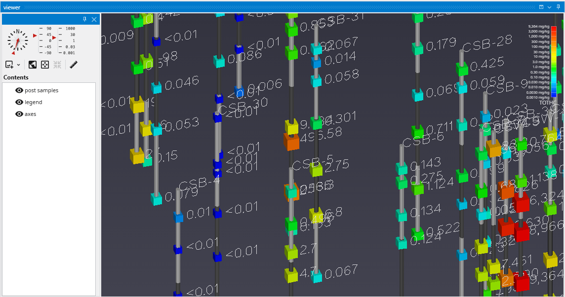
Double click on post samples to open its Properties window. Select Analytic and Stratigraphic Modeling\railyard.apdv and change the Z Scale to 5 on the Application window or Application Properties.

to show the following in the viewer.

post samples has many options for displaying this type of data (also applicable to PGF, GEO, AIDV). These include (but are not limited to):

• displaying the data as colored tubes (with or without spheres/glyphs)
• using different glyphs to represent each sample (a sphere is the default glyph)
• changing the diameter of glyphs or tubes based on the data magnitudes
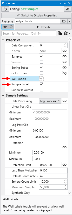
• labeling the samples and/or borings

Let’s see the four options above:

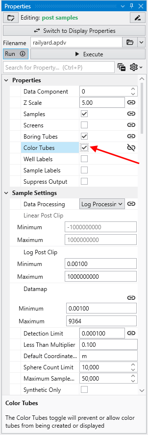
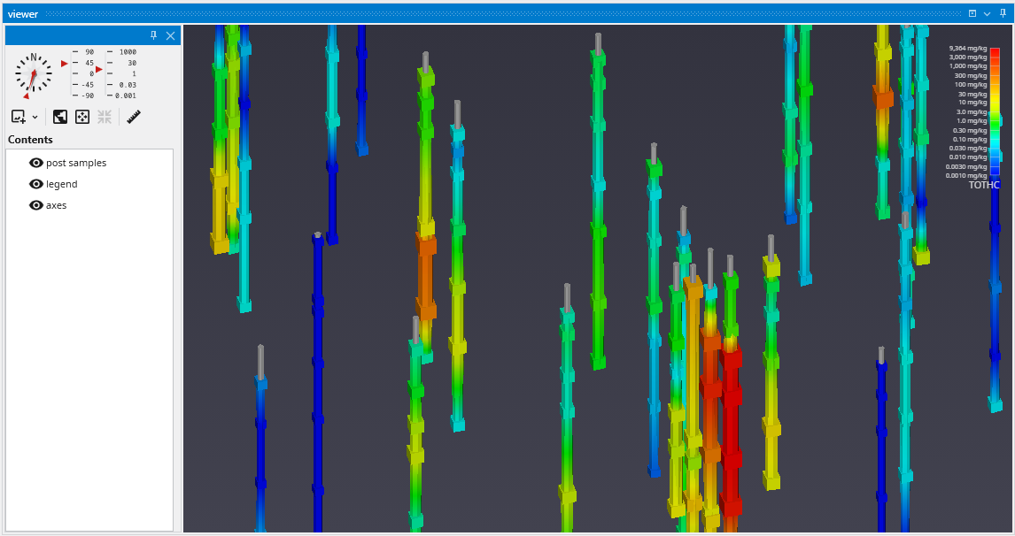
It is easy to display colored tubes. You can scroll down to the Color Tubesoption in the “Properties” cagtegory.

Check the Color Tubes option:

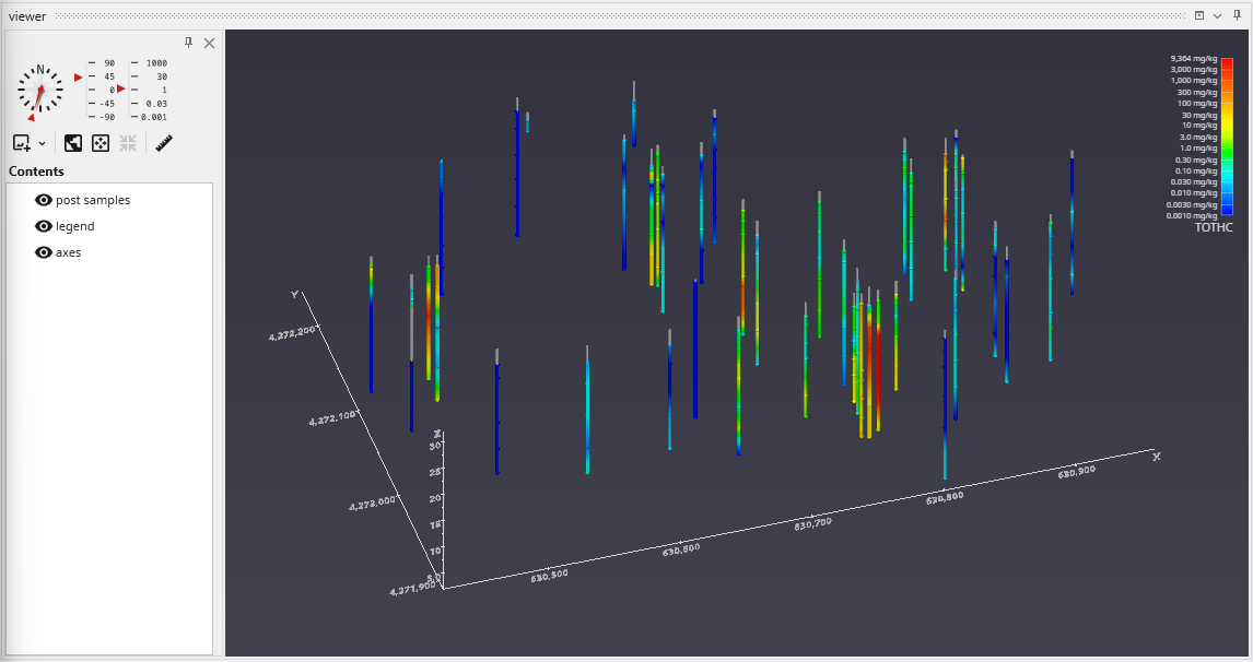
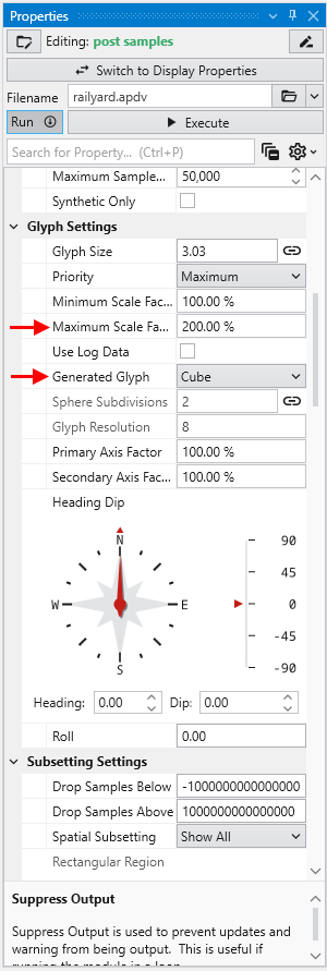
To change glyphs is incredibly simple. We just go to the Glyph Settings, and we’ll change the Generated Glyph to be Cube instead of the default Sphere, and we’ll also set the Maximum Scale Factor to be 200%

Since we’ve still left colored tubes on, our viewer shows:

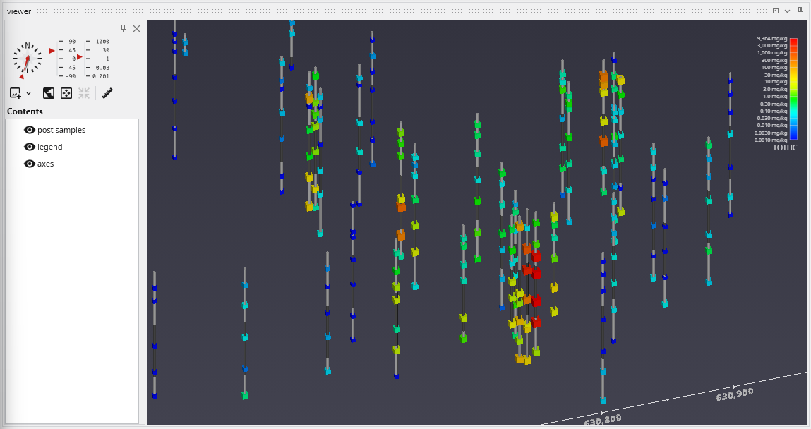
Before we make any other changes let’s uncheck the Color Tubes option again which will change our view to be:

Finally, we’ll add labels at each sample and the top of the borings:

When working with dense datasets, sample labels can become cluttered and difficult to read. The post samples module includes label subsetting features to resolve this by intelligently blanking labels to improve clarity. This functionality is controlled by the Label Subsetting option in the Label Settings category.

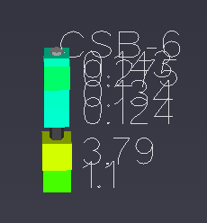
For example, if you set the Z Scale in the Application Properties to 1.0 and zoom in on a boring with dense data, such as CBS-6, you will see the problem of overlapping and unreadable labels:

To resolve this, locate the Label Subsetting option and set it to Blank Labels.

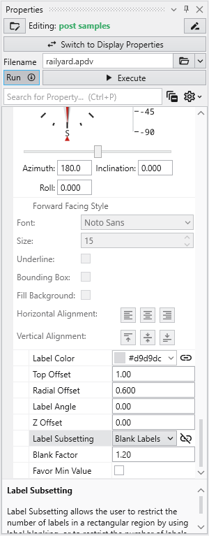
By default, Label Subsetting is set to None. Changing it to Blank Labels enables collision detection, which hides lower-priority labels that overlap with higher-priority ones. Label priority is determined by the sample’s value, with higher values taking precedence. Well labels, if enabled, are always given the highest priority. The result is a much cleaner and more informative visualization.

Before: No Blanking	After: Blanking Enabled

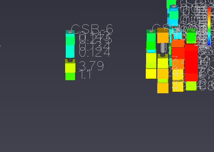
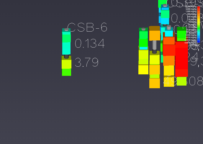
You can further refine the display using the following settings:

• Blanking Factor: This setting controls the size of the buffer around each label used for collision detection. Increasing this value creates more space around labels, potentially blanking more of them.
• Boring Min/Max: This mode displays only one sample label per boring, either the one with the highest or lowest value. The Favor Min Value toggle determines which is shown.

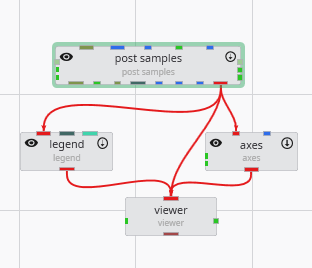
AIDV files represent analyte data which is measured over an interval. The data is inherently collected along borings. Boring IDs are required in the file, and post samples will draw the borings as well as the sample intervals.

Create the following application. It is identical to the application used for APDV files.

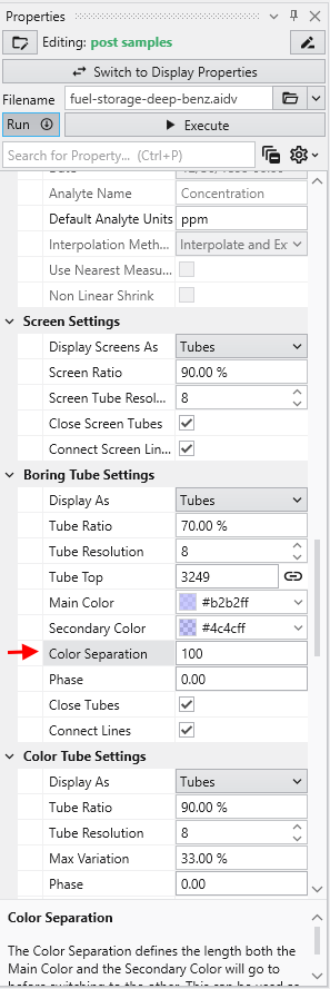
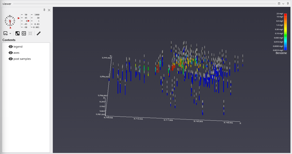
Let’s read the file in Studio Projects: Analytical (Contaminant) Modeling\fuel-storage-deep-benz.aidv

By default, post samples will display AIDV files as intervals of colored tubes representing the top and bottom of each sample screen.

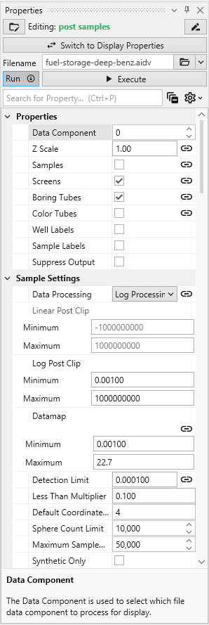
This dataset spans 779 feet in Z. One of our default settings is “Color Separation which colors the borings light-and-dark grey alternating every 10 units (feet) in depth. We want to change that parameter to be 100 feet for this data.