2D Estimation: Instance Modules Now let’s see just how fast we can instance the modules to create a useful application. In the Modules section of the Application network window, type 2 This will show all modules beginning with the number 2. From this filtered list we can instance any of these modules by double-clicking on them. However, we can get the first one, 2d estimation by hitting Enter. Do that.
We'll now connect these modules. Connections determine how data flows or is shared among modules, and affects the modules' order of execution. Use the
Let's execute the analysis module, 2d estimation, in order to produce a model based on the data file we will select. You will need to have installed
With the kriging interpolation results from 2d estimation, the next step is to refine the visualization. This can be accomplished by subsetting the
Subsections of Workbook 2: 2D Estimation of Analytical Data
2D Estimation: Instance Modules
Now let’s see just how fast we can instance the modules to create a useful application. In the Modules section of the Application network window, type 2
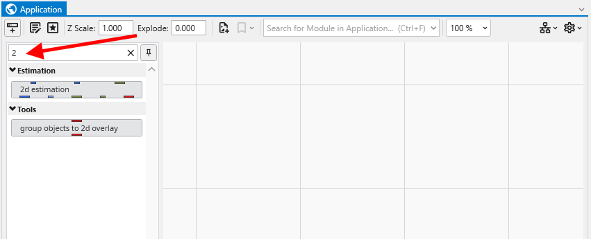
This will show all modules beginning with the number 2. From this filtered list we can instance any of these modules by double-clicking on them. However, we can get the first one, 2d estimation by hitting Enter. Do that.
When you hit enter, it also clears the filter (search) field.
Now type p. Double-click on plume, ~5th in the list.
Since we didn’t hit enter, we need to clear the p and now type e. Double-click on external edges, 7th in the list.
Finally, backspace or clear the e and type l for legend, finding it as the 5th module and double click on it too.
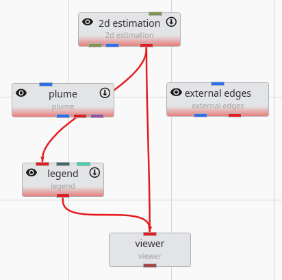
You may need to pan in the application to see our application should be:
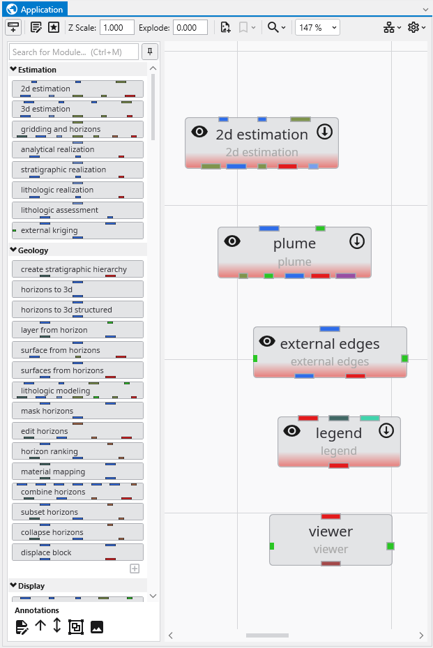
We’ll now connect these modules. Connections determine how data flows or is shared among modules, and affects the modules’ order of execution. Use the left mouse button to drag from one port to another to connect them.
We could leave these modules in their current positions, but let’s move them around so they better match how we want the data to flow. Adjust the positions to approximately match:
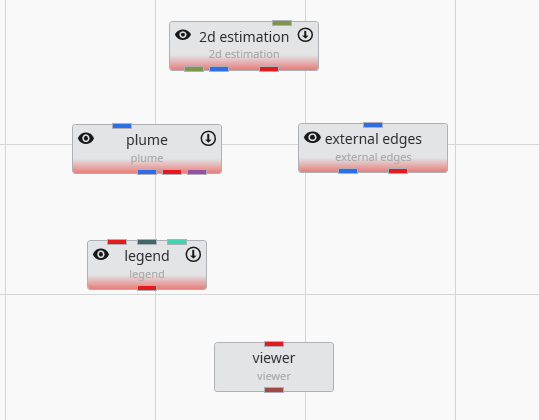
Then connect a few of them as shown below.
The method of connecting modules is detailed in the topic Connecting and Disconnecting Modules.
Info
The order in which we instance and connect modules is, with the exception of certain array connections, unimportant. We could have instanced and connected these modules in any order.
We are not connecting all of the modules at this time since we want to examine the simplest 2D kriging applications first and then make it more complex.
Let’s execute the analysis module, 2d estimation, in order to produce a model based on the data file we will select. You will need to have installed the Studio Projects specific to the version of Studio you have installed.
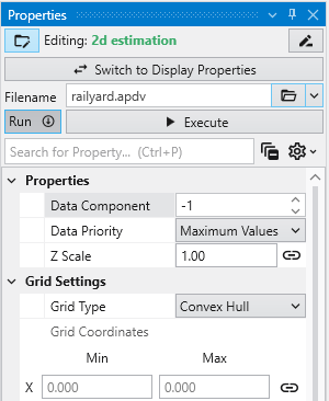
- First, double-left-click on 2d estimation to open its properties so you can see the window below
- Click on the Open button to the right of Filename and browse to Studio Projects/Analytic and Stratigraphic Modeling and choose railyard.apdv
- Then click “Execute”.
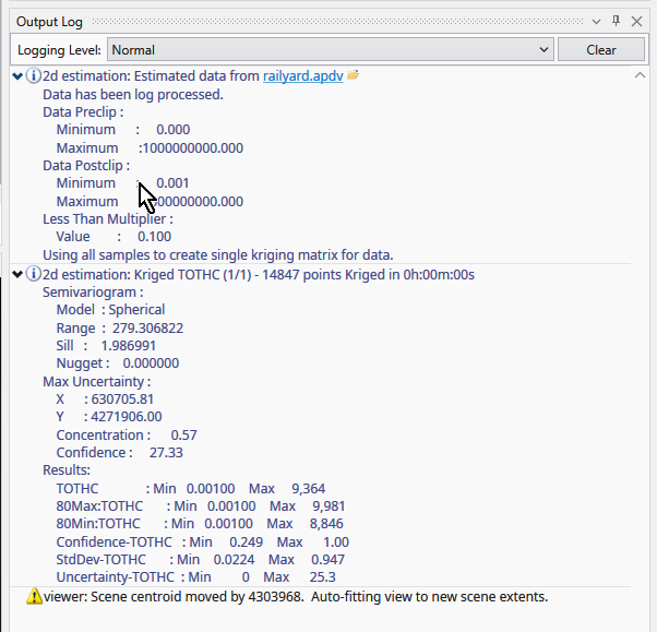
2d estimation reads the analyte (e.g. chemistry) data and begins the kriging process. In a very short time, it calculates the estimated concentrations for the grid we selected.
While it runs, 2d estimation prints messages to the Information Window such as percentage completion.
When it is done, the Output Log will show two lines, which when expanded will display:
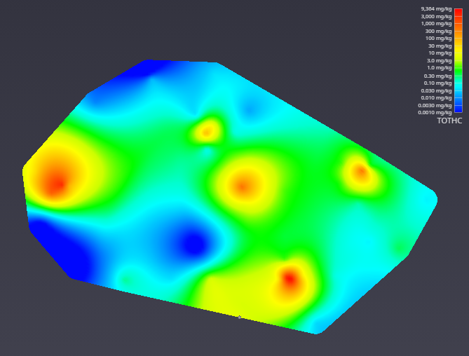
The viewer will promptly display a top view of the surface we have estimated. Your viewer should look like this:
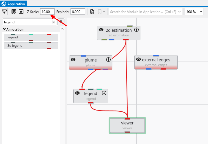
In the Application window, please change the Z Scale to 10. This will create an artificial topography to our surface where elevations correlate to concentration.
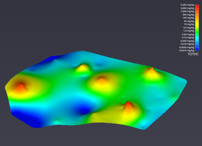
With a simple rotation of our model we now have
With the kriging interpolation results from 2d estimation, the next step is to refine the visualization. This can be accomplished by subsetting the output to display only the regions that fall within a specific value range.
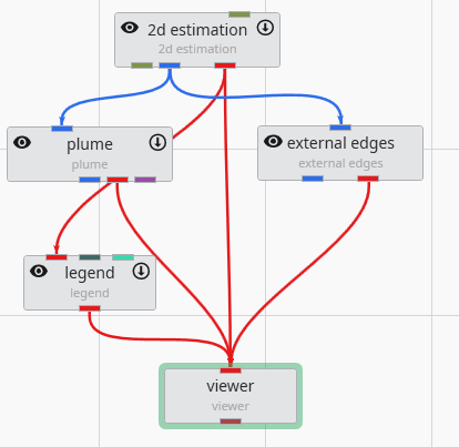
To begin, connect the 2d estimation module to a plume module, and then connect the plume module to the viewer. This directs the data flow through the plume module, which will perform the subsetting operation before rendering the final output.
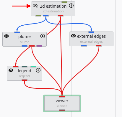
Initially, the viewer’s output may appear unchanged. This is because the 2d estimation and plume modules are rendering overlapping geometry. To isolate the output from plume, you can toggle the visibility of the 2d estimation module. Click the eye icon on the 2d estimation module in the Application Network to hide its output. This feature is essential for debugging complex applications, allowing you to focus on the output of specific modules.
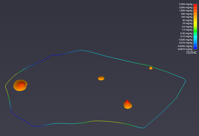
After hiding the upstream module, the viewer updates to show only the geometry from the plume module. The visualization is now more informative, displaying only the areas of interest where the TOTHC value is above 3.06. This default level was automatically determined from the data entering the plume module as a starting point for you to estimate a suitable value in the data range.
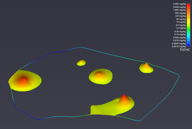
You can easily customize this filtering behavior. To demonstrate, select the plume module by double-clicking it. In the Properties window, set the Subsetting Level to 100.
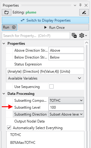
The viewer immediately reflects these changes. As a result, it now renders only the regions with a TOTHC value above 100, effectively further reducing the areas of high concentration. This feature allows you to interactively explore your data and isolate different phenomena within the dataset.