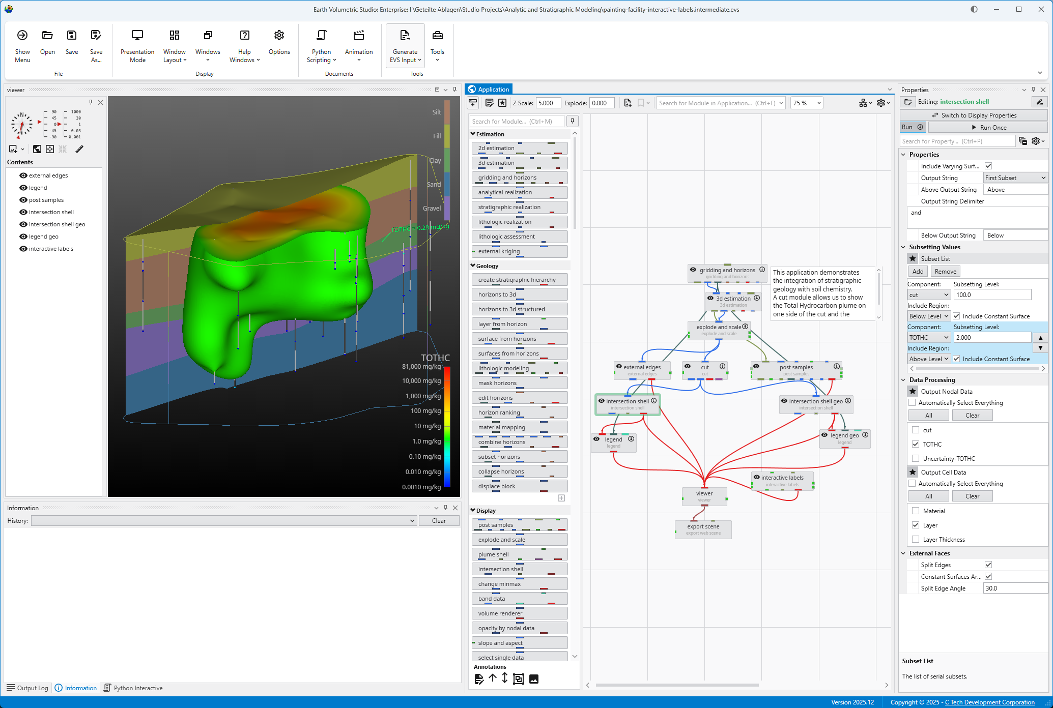
Let’s load an application to get an idea of how EVS works. Browse to Find and double click the file “painting-facility-interactive-labels.intermediate.evs”. The application will run and in less than one minute you will see:
Transformations with the Mouse Now that we have an application loaded, let’s investigate the many ways we can interact with it. Rotate the model Hold down the left mouse button and move the mouse pointer in various directions. The model rotates. Vertical motions rotate the model about a horizontal axis. Horizontal motions rotate the model about a vertical axis. Roll is suppressed so that mouse rotations always keep vertical objects (e.g. telephone poles) vertical. Scale (zoom) the model
Transformations with the Azimuth and Inclination Controls Azimuth and Inclination controls are available in two places and gives us more precise ways to transform (scale, pan and rotate) an object: The viewer’s Properties window. The viewer’s slide-out properties in the Viewer window. Double click on the viewer module to open the Properties window with view controls including sliders and an array of buttons. These controls allows you to instantly select a view from any azimuth and inclination. For a given (positive) inclination, selecting different azimuth buttons is equivalent to flying to different compass points on a circle at a constant elevation. The azimuth buttons are the direction from which you view your objects. (i.e. 180 degrees views the objects from the south). An inclination of 90 degrees corresponds to a view from directly overhead, 0 degrees is a view from the horizontal plane (side view) and -90 degrees is a view from the bottom.
At any time after modules have run, you can quickly obtain basic statistical and model extents data merely by double left mouse clicking on any FIELD (blue) output port. Let’s demonstrate this by using the second output port of the cut module When we double-click here, the following information appears in the Properties window.
Before we end this first workbook, let's interact with this application in another way.
Let's exit EVS.
EVS Project Structure for Maximum Portability
Create a 'project' folder with all of your data in one or more subfolders under that folder (any number of levels deep). As long as you don't put your
Subsections of Workbook 1: Earth Volumetric Studio Basics
Let’s load an application to get an idea of how EVS works.
Browse to
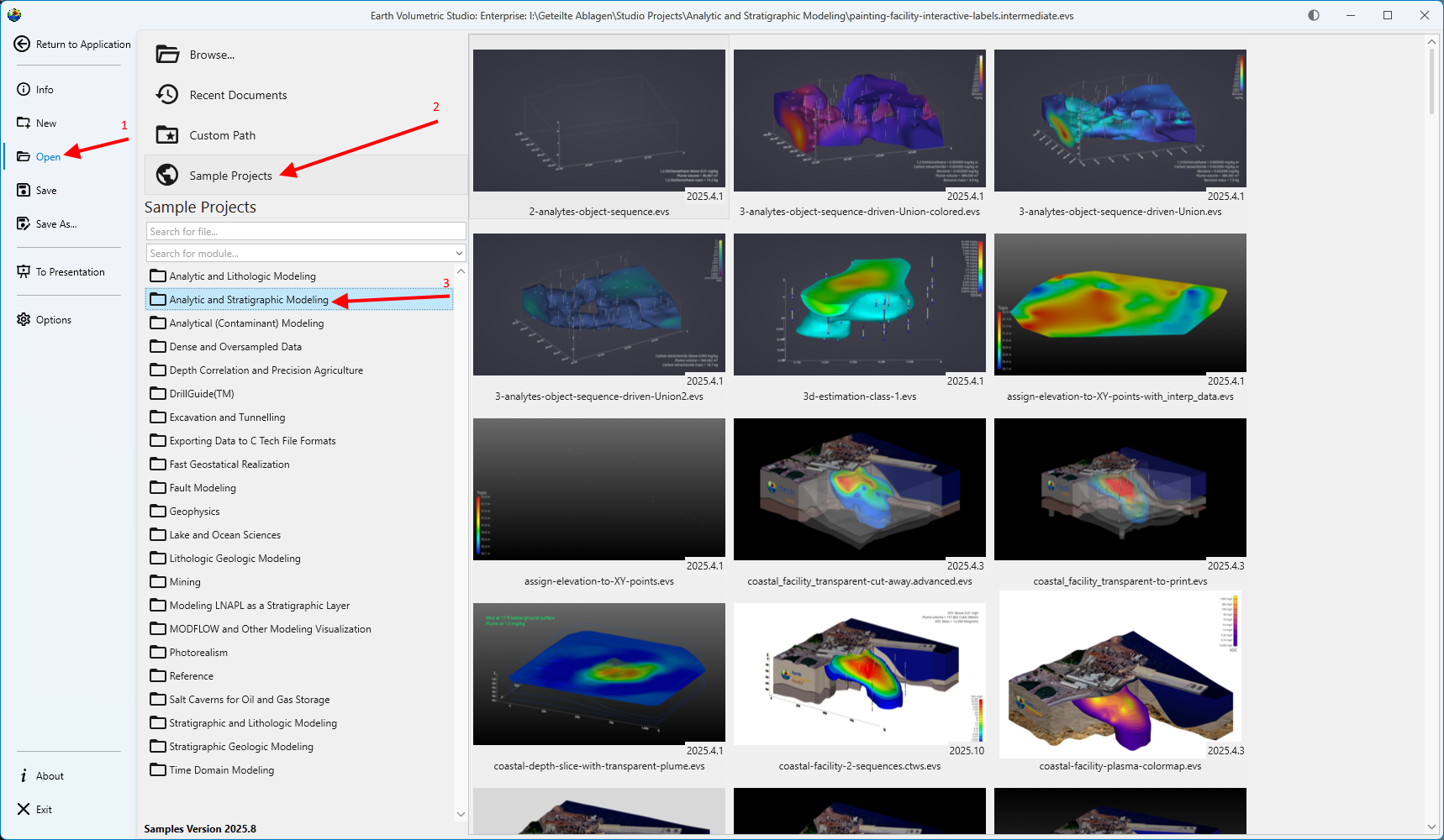
Find and double click the file “painting-facility-interactive-labels.intermediate.evs”.
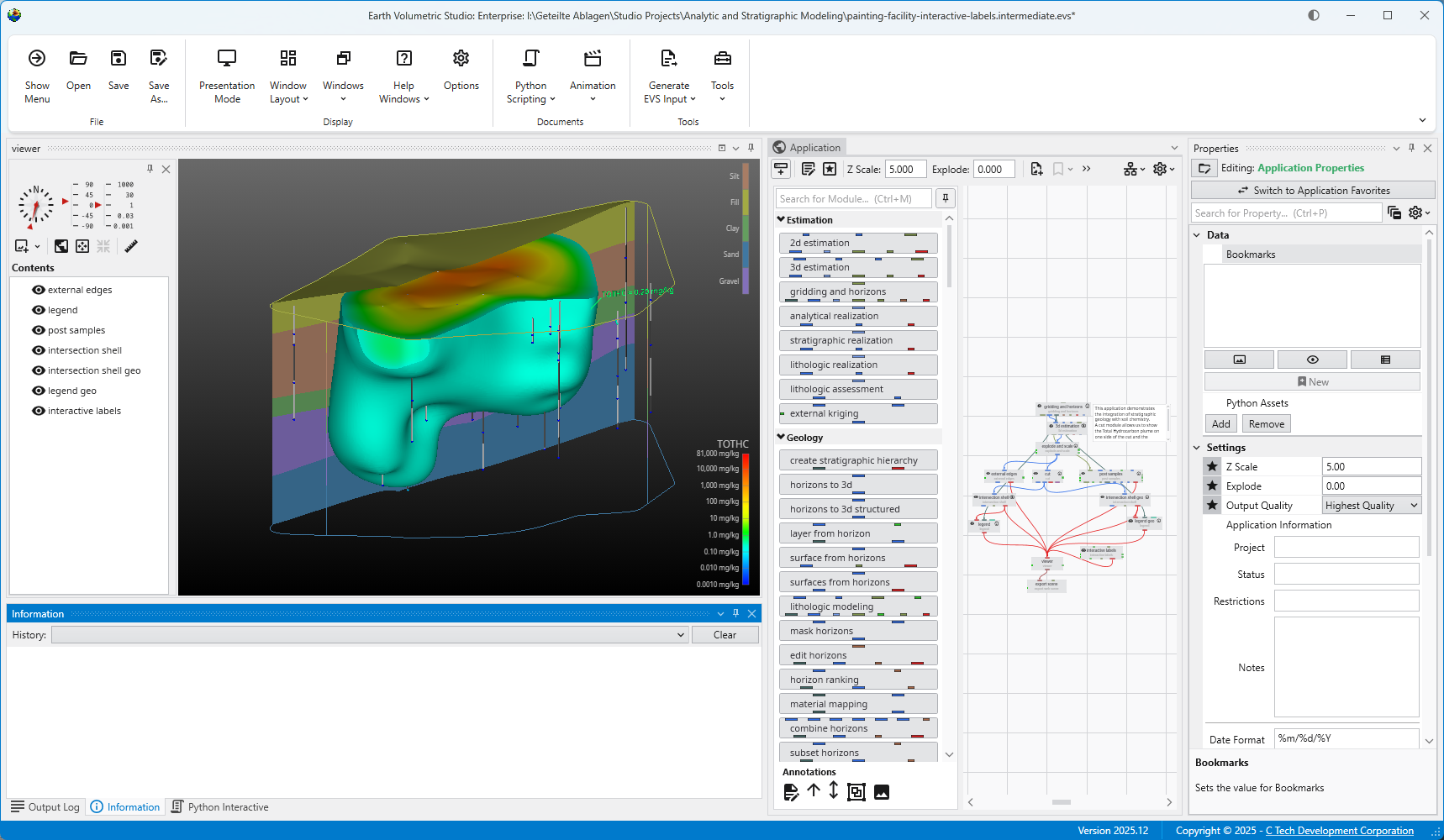
The application will run and in less than one minute you will see:
For more on opening applications see the topic Open Files.
Transformations with the Mouse
Now that we have an application loaded, let’s investigate the many ways we can interact with it.
Rotate the model
- Hold down the left mouse button and move the mouse pointer in various directions. The model rotates.
- Vertical motions rotate the model about a horizontal axis.
- Horizontal motions rotate the model about a vertical axis.
- Roll is suppressed so that mouse rotations always keep vertical objects (e.g. telephone poles) vertical.
Scale (zoom) the model
- The wheel on wheel mice also zooms in and out.
- Alternate method:
- Hold down both the Shift key and the left mouse button (or the middle button alone).
- Keeping the Shift key and mouse button held down, move the mouse pointer downward or to the left. As we do, the model scales down. Moving the mouse pointer upward or to the right scales up.
Move (Translate or Pan) the model
- Hold down the right mouse button and drag the object up, down, and around, then center the model.
| Mouse-controlled operations | What to do |
|---|---|
| Translate | Drag the object with the right mouse button (RMB) |
| Rotate | Drag the object with the left mouse button (LMB) |
| Scale | Use the wheel to zoom in and out |
or
Hold down the Shift key and drag the object with the left mouse button (Shift-LMB)
or
Use the middle mouse button or wheel as a button without Shift |
Transformations with the Azimuth and Inclination Controls
Azimuth and Inclination controls are available in two places and gives us more precise ways to transform (scale, pan and rotate) an object:
- The viewer’s Properties window.
- The viewer’s slide-out properties in the Viewer window.
Double click on the viewer module to open the Properties window with view controls including sliders and an array of buttons. These controls allows you to instantly select a view from any azimuth and inclination. For a given (positive) inclination, selecting different azimuth buttons is equivalent to flying to different compass points on a circle at a constant elevation. The azimuth buttons are the direction from which you view your objects. (i.e. 180 degrees views the objects from the south). An inclination of 90 degrees corresponds to a view from directly overhead, 0 degrees is a view from the horizontal plane (side view) and -90 degrees is a view from the bottom.
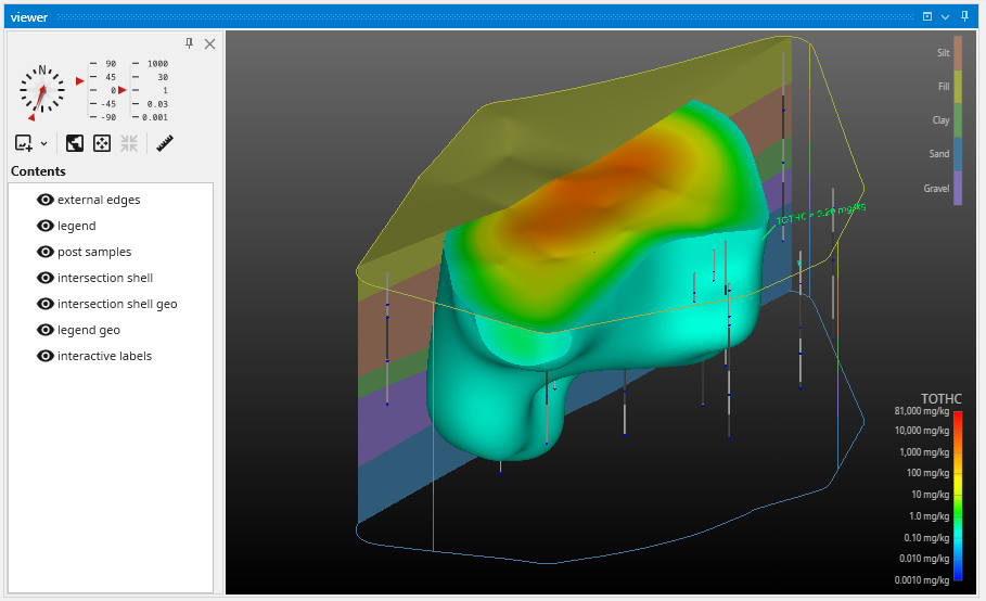
c. Use the Azimuth and Inclination Panel to obtain a specific view by setting the scale slider and inclination slider to desired settings and click once on the desired azimuth button. If you choose a scale of 1.0, an Inclination of 30 degrees and an azimuth of 200 degrees
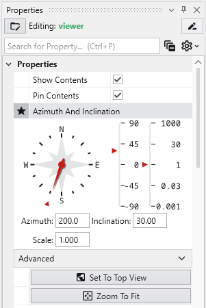
The viewer will show:
The Advanced options provide the ability to allow rotations about a user defined center, as opposed to the default center of the objects, which is chosen by EVS. Additionally you can apply a ROLL to the view which will make vertical objects (such as the Z axis) not appear vertical. If you do not see the options, click on the Advanced category in the Properties window to expand them.
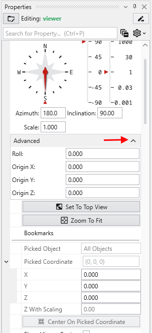
Below the Advanced options, there are three buttons
- Set to Top View: Returns the model view to Azimuth 180, Inclination 90 and Scale of 1.0
- Zoom To Fit: Returns the Scale to 1.0
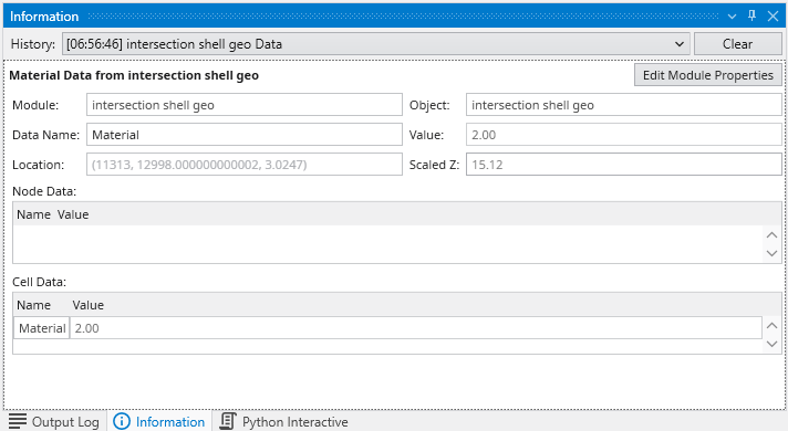
- Center On Picked: This button is normally inactive, but is activated by probing with CTRL-Left mouse on any object in the view. The default center of an object shown in our viewer is midway between the min-max of the x, y and z dimensions. This button then causes the view to recenter on the selected point. When you pick a point on an object, the following information is displayed in the Information window.
The Perspective Mode toggle switches to Perspective (vs. Orthographic) viewing. In perspective mode, parallel lines no longer appear parallel but instead would point to a vanishing point.
The Field of View determines the amount of perspective. Larger values result in more perspective distortion.
The Render selection allows you to choose between OpenGL and Software renderers. On some computers with minimal graphics cards Software renderer may perform better or be more stable.
Auto Fit Scene: The choices here include:
- On Significant Change: This is the default behavior which causes the view to recenter and rescale if the extents of the view would change significantly. Otherwise the view is unaffected.
- On Any Change: This causes the view to recenter and rescale if the extents of the view changes at all
- Never: The view will not change if objects change.
The Window Sizing options
- Fit to Window: The view size is determined by the size of the viewer window
- Size Manually: The view size is set in the Viewer Width and Height type-ins below to a specific size. The viewer then has scroll bars if the view size exceeds the window size.
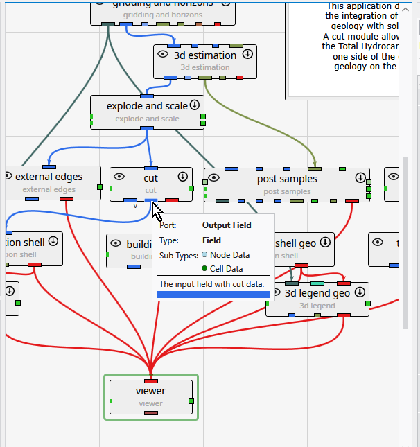
At any time after modules have run, you can quickly obtain basic statistical and model extents data merely by double left mouse clicking on any FIELD (blue) output port.
Let’s demonstrate this by using the second output port of the cut module
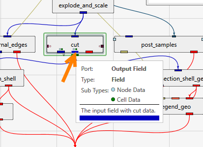
When we double-click here, the following information appears in the Properties window.
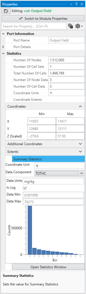
This quickly tells us that this port has a model with the following data and coordinate extents
- 211,200
- 181,779 cells
- We can select any of the three nodal data (TOTHC is shown)
- The X, Y & Z Minimum, Maximum and Extents are provided
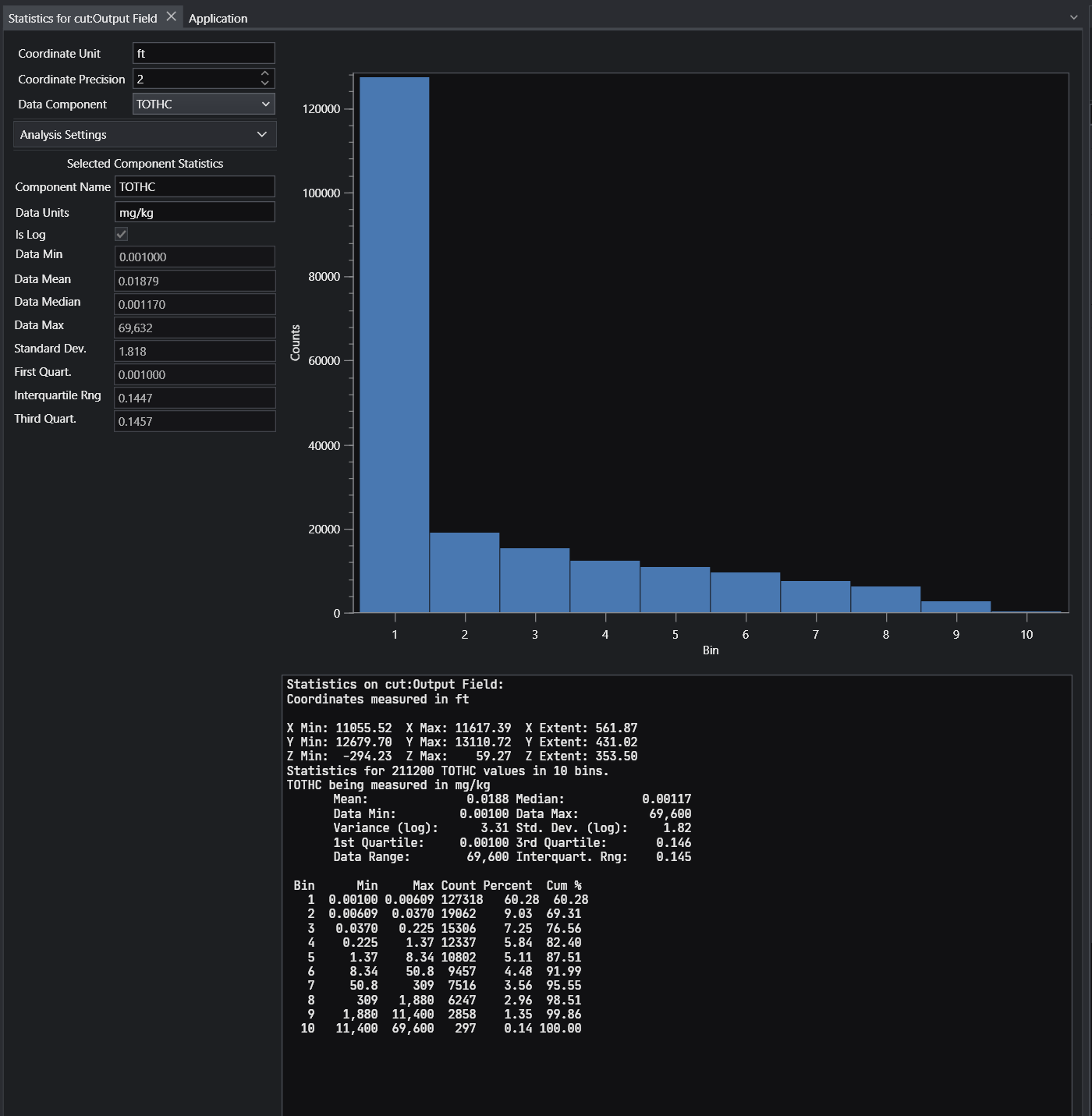
For more comprehensive statistical analysis of the nodal data, click on the “Open Statistics Window” button, and the following appears.
Before we end this first workbook, let’s interact with this application in another way.
In the Application window, double click on the intersection_shell module, and you will see a green border around it. This green border designates the selected module whose properties are available for editing.
This will open its Properties in the Properties window in the upper right. In this application, intersection_shell is performing two tasks. It is cutting the model using information provided by the cut module and it is also subsetting what remains by Total Hydrocarbon (TOTHC) level. It might seem strange at first that the cut module isn’t actually cutting the model. But if it did, it would only provide one side or the other. By giving us data that is the “signed” distance from the specified cutting plane, we are able to use cut’s data to create the cut for the front side giving us the plume and the back side giving us the geologic layers. We can also offset any distance from the theoretical cutting plane without actually moving the cutting plane, but only changing the “cut” Subsetting level. In fact, in this application we’re cutting 100 feet from the specified cutting plane.
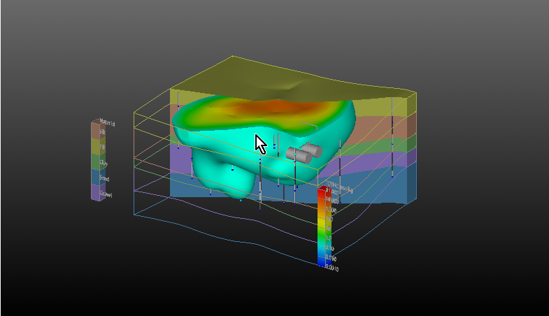
Change the TOTHC Subsetting Level to be 2.0 and your view should look like this:
You can continue to experiment and see that you can view any subsetting level in less than a second.
Let’s exit EVS.
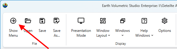
Open the Menu using the Show Menu button in the upper right corner. Select Exit at the bottom. Alternatively, exit EVS using the regular close icon at the upper right on the main window.
EVS exits after displaying a confirmation message.
If you close the main window using the X in the upper left, it will prompt you similarly.
You have now completed Workbook 1.
Create a “project” folder with all of your data in one or more subfolders under that folder (any number of levels deep). As long as you don’t put your applications more than 2 levels deep inside of the project folder, everything will be relative, and moving the project folder (as a whole) will always “just work”.
An example would be:
- drive\some\path
- project
- applications
- data
- data sub 1
- data sub 2
- project
Alternatively, the most portable EVS Application is one where all of the data is packaged.