When a volumetric model is created, we generally use geostatistics to estimate (interpolate and extrapolate) data into the volume based on sparse measurements. The algorithm used is called kriging, which is named after a South African statistician and mining engineer, Danie G. Krige who pioneered the field of geostatistics. Kriging is not only one of the best estimation methods, but it also is the only one that provides statistical measures of quality of the estimate.
The basic methodology in kriging is to predict the value of a function at a given point by computing a weighted average of the known values of the function in the neighborhood of the point. The method is mathematically related to regression analysis. Both derive a best linear unbiased estimator, based on assumptions on covariances and make use of Gauss-Markov theorem to prove independence of the estimate and error.
The combination of kriging and volumetric modeling provides a much more feature rich model than is possible with any model that is limited to external surfaces and/or simpler estimation methods such as IDW or FastRBF. It allows us to perform volumetric subsetting operations and true volumetric analysis, and we can defend the quality of our models based on the limitations of our data.
In the coal mining industry, we can determine the quantity and quality of coal and its financial value. We can assess the amount and extraction cost of excavating overburden layers that must be removed or whether it is more cost effective to use tunneling to access the coal.
In the field of environmental engineering, where our software was born, volumetric modeling allows us to determine the spatial extent of the contamination at various levels as well as compute the mass of contaminant that is present in the soil, groundwater, water or air. During remediation efforts, this is critical, since we must confirm that the mass of contaminant being removed matches the reduction seen in the site, otherwise it is a clue that during the site assessment we have not found all the sources of contamination. This can result in remediation efforts which create contamination in some otherwise clean portions of the site.
The kriging algorithm provides us with only one direct statistical measure of quality, and that is Standard Deviation. However, C Tech uses Standard Deviation to compute three additional metrics which are often more meaningful. These are:
Standard Deviation
Inherent in the kriging process is the determination of the expected error or Standard Deviation at each estimated point. As we approach the location
Confidence
The Confidence values are the answer to a question, and the wording of the question depends on whether you are Log Processing your data or not.
Uncertainty
At first glance, confidence seems to be a reasonable measure of site assessment quality. If the confidence is high (and we are asking the right questi
Min Max Estimate
Both krig_2d and 3d estimation include the ability to compute the Minimum and Maximum Estimate, which is computed using the nominal estimates and sta
Subsections of Workbook 6: Geostatistics Overview
Inherent in the kriging process is the determination of the expected error or Standard Deviation at each estimated point. As we approach the location of our samples, the standard deviation will approach zero (0.0) since there should be no error or deviation at the measured locations.
The units of standard deviation are the same as the units of your estimated analyte.
The figure below shows why one standard deviation corresponds to 68% of the occurences, whereas three sigma (standard deviations) covers 99.7%
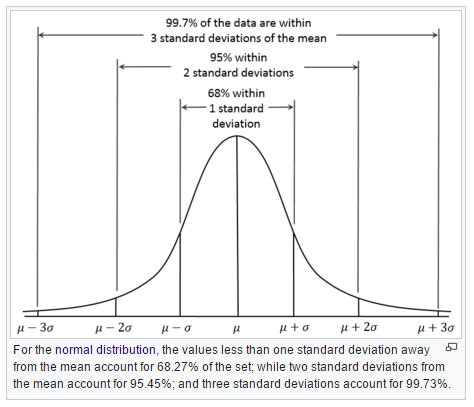
At a particular node in our grid, if we predict a concentration of 50 mg/kg and have a standard deviation of 7 mg/kg , then we can say that we have a ~68% confidence that the actual value will fall between 43 and 57 mg/kg.
The computation of the expected Minimum and Maximum estimates for a given Confidence level is what our Min/Max Estimate provides.
The Confidence values are the answer to a question, and the wording of the question depends on whether you are Log Processing your data or not.
- For the “Log Processing” case the question is: What is the “Confidence” that the predicted value will fall within a factor of “Statistical Confidence Factor” of the actual value?
- For the “Linear Processing” case, the question is: What is the “Confidence” that the predicted value will fall within a +/- tolerance “Statistical Confidence Tolerance” of the actual value?
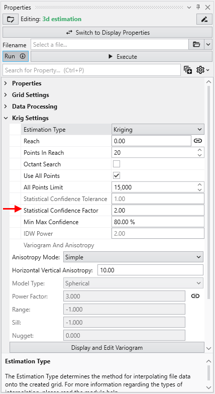
So if your “Statistical Confidence Factor” is 2.0 as shown for a Log Processing case above, the question is:
What is the “Confidence” that the predicted value will fall within a factor of 2.0 of the actual value?
The confidence is affected by your variogram and the quality of fit, but also by the range of data values and the local trends in the data where the Confidence estimate is being determined.
If your data spans several orders of magnitude, the confidences will be lower and if your data range is small the confidences will be higher depending also on the settings you use.
If the “Statistical Confidence Factor” were set to 10.0, because we are working on a log10 scale, EVS would take the log10 of the Statistical Confidence Factor (the value was 10, so the log is 1.0). It then compares the log concentration values and a corresponding standard deviation that was calculated for every node in our domain. For log concentrations, one unit is a factor of ten, therefore we are asking what is the probability that we will be within one unit. Above, where the Statistical Confidence Factor is 2.0, the questions would have been: What is the confidence that the predicted concentration will be within a factor of 2 of the actual concentration?
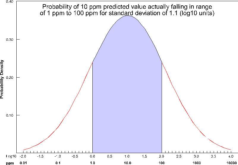
The actual calculation to determine confidence requires the standard deviation of the estimate at a node, and the Statistical Confidence Factor. The figure below shows the confidence (as the shaded area under the “bell” curve) for a Statistical Confidence Factor of 10 at a node where the predicted concentration was 10 ppm (1.0 as a log10 value) and the standard deviation for this point was 1.1 (in log10 units). For this example, the confidence would be ~64%, which means that 64% of the time, the value would lie in the shaded region.
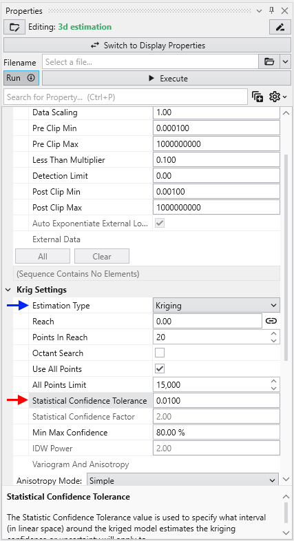
For example, consider the case where we are estimating soil porosity, and the input data values are ranging from 0.12 to 0.29. We would want to use “Linear Processing”, and since our values fall within a tight range of numbers we might want to use a “Statistical Confidence Tolerance” that was 0.01. The confidence values we would compute would then be based upon the following question:
What is the “Confidence” that the predicted porosity value will be within 0.01 of the actual value?
If we were careless and used a “Statistical Confidence Tolerance” of 1.0 all of our confidences would be 100% since it would be impossible to predict any value that would be off by 1.0.
However, if we used a “Statistical Confidence Tolerance” of 0.0001, it is likely that our confidence values would drop off very quickly as we move away from the locations where measurements were taken.
At first glance, confidence seems to be a reasonable measure of site assessment quality. If the confidence is high (and we are asking the right question), we can be assured of the reasonableness of the predicted values. You might be tempted to collect samples everywhere that the confidence was low, and if you did, your site would be well characterized.
But, there is a better, more cost-effective way. Instead of focusing on every place where confidence was low, we could focus on only those locations where there was low confidence and where the predicted concentration was reasonably high. We make that easy by providing the Uncertainty.
In EVS, uncertainty is high where concentrations are predicted to be relatively high (above the Clip Min), but the confidence in that prediction is low. If the goal is to find the contamination, using uncertainty allows for more rapid, cost effective site assessment. Uncertainty is the core of our DrillGuideTM technology which performs successive analyses using the location of Maximum Uncertainty to select new locations for sampling on each analysis iteration.
NOTICE: Uncertainty values should be considered unitless and their magnitudes cannot directly be used to assess the quality of a site assessment. Please observe the following precautions:
- Use Uncertainty as it was intended, as a guide to locations needing additional characterization.
- Do not use Uncertainty values directly to assess the quality of a site assessment
- A 50% reduction in Uncertainty magnitude cannot be construed as a 50% improvement in site assessment.
Our training videos cover the use of DrillGuide and how to properly use and interpret Uncertainty.
Both krig_2d and 3d estimation include the ability to compute the Minimum and Maximum Estimate, which is computed using the nominal estimates and standard deviations at every grid node based upon the user input Min-Max Plume Confidence.
The issue with our MIN or MAX plumes is that they represent the statistical Min or Max at every point in the grid. It is quite unrealistic to believe that you could possibly have a case where you’d find the actual concentration would trend towards either the Min or Max at all locations.
C Tech’s Fast Geostatistical Realizations^®^ (FGR^®^) creates more plausible cases (realizations) which allow the Nominal concentrations to deviate from the peak of the bell curve (equal probability of being an under-prediction as an over-prediction) by the same user defined Confidence. However, FGR^®^ allows the deviations to be both positive (max) and negative (min), and to fluctuate in a more realistic randomized manner.
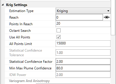
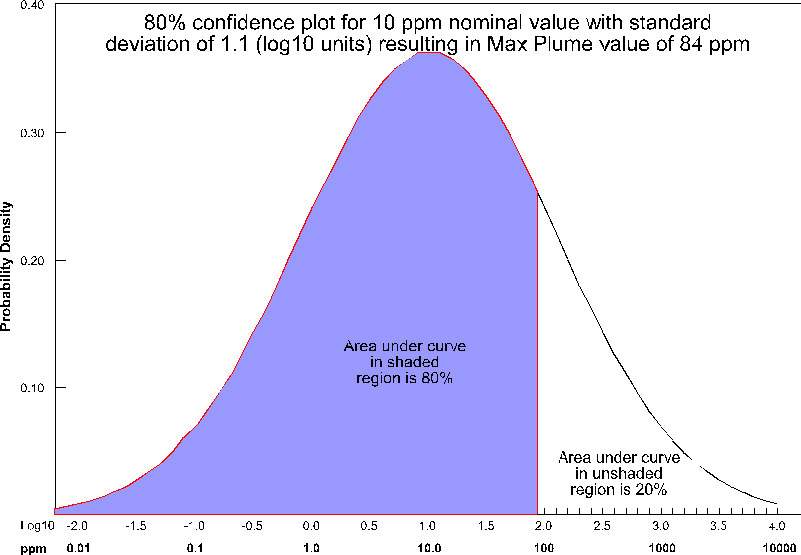
For the case of Max Plume and 80% confidence, at each node, a maximum value is determined such that 80% of the time, the actual values will fall below the maximum value (for that nominal concentration and standard deviation). This process is shown below pictorially for the case of a nominal value of 10 ppm with a standard deviation of 1.1 (log units). For this case, the maximum value at that node would be ~84 ppm. This process is repeated for every node (tens or hundreds of thousands) in the model.
Note that for this plot, the entire left portion of the bell curve is shaded. If we were assessing the minimum value, it would be the right side. Statistically, we are asking a different type of question than when we calculate confidence for our nominal concentrations.
If this Confidence value were set to ~81% then we would be adding one standard deviation to the nominal estimate to create the Max and subtracting one standard deviation to create the Min. The higher you set the Min-Max Plume Confidence the greater the multiplier for standard deviations which are added/subtracted to create the Max/Min.
Even though Min & Max Estimates may not be realistic “realizations” of a likely site state, they still provide the best technique to determine when your site is adequately characterized. Some sites may have very complex contaminant distributions and high gradients while others may be very simple. Applying a single standard for sampling based on fixed spacing will never be optimal.
It is up to the regulators and property owners to determine the ultimate criteria, but generally having the ability to assess the variation in the expected plume volume and the corresponding variation in analyte mass within, provides the best metric for assessing when a site has been sufficiently characterized.