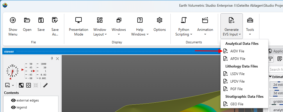
Begin by selecting the “Generate EVS Input” button in the Main Toolbar, and select AIDV File.

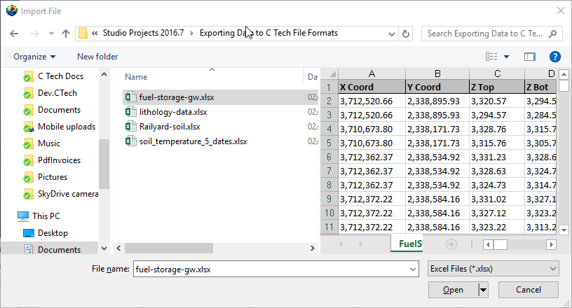
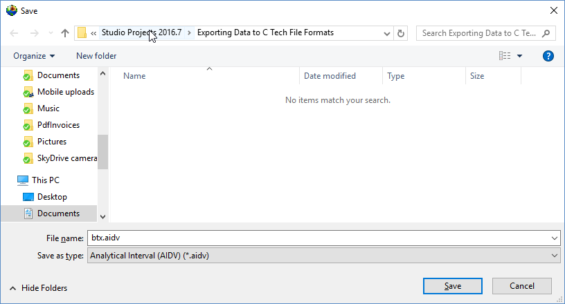
Let’s browse to the folder shown and select the file fuel-storage-gw.xlsx

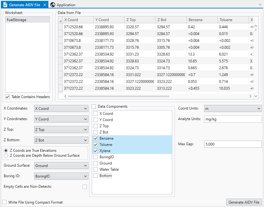
You’ll need to select the appropriate table in the file. Some may have several, this one has only one named FuelStorage. Once you do, the program will attempt to automatically choose settings for you, but as you can see below, it isn’t perfect.

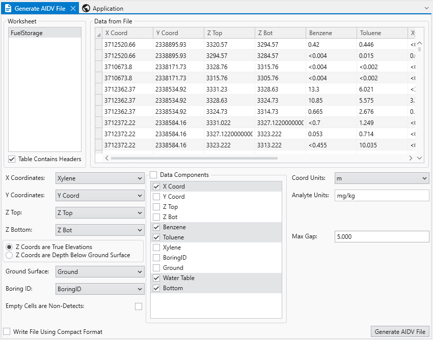
Since Xylene starts with the letter “X”, it was chosen as the X Coordinate. This is clearly wrong, however, everything else along the left side is correct. By default, the Data Components list will select whatever is left over. Sometimes this is handy, but often, and in this case it is excessive. This excel table includes water table and bottom of model elevations that we will want for a .GEO file, but not for the AIDV file. So we’ll need to make quite a few changes.

It also can’t know the correct units for your analytes nor your coordinate units. It is your responsibility to make sure these are correct or change them.

The last thing you MUST do is determine and choose a Max Gap parameter. This parameter takes some understanding to properly determine. I’ve looked at this excel file in detail and the screen intervals vary from 0.26 to 35.1 meters in length. The Max Gap parameter is the longest length we will allow to be converted into a single point when we convert intervals to points for kriging. I would recommend setting it to 5 for this data file. That means that any interval less than 5 meters will be represented by a single point at the center of the interval. Intervals longer than 5 meters will be represented by two or more points. Choosing a value too small will create oversampling along the Z direction and too large can result in plumes which become disconnected in Z. Fortunately there tends to be a large range of reasonable values. For this dataset, I expect that good results can be obtained with values ranging from 1 to 12.

With all of our settings correct as shown above, all we need to do is click the Generate AIDV File button, and let’s call the file btx.aidv.

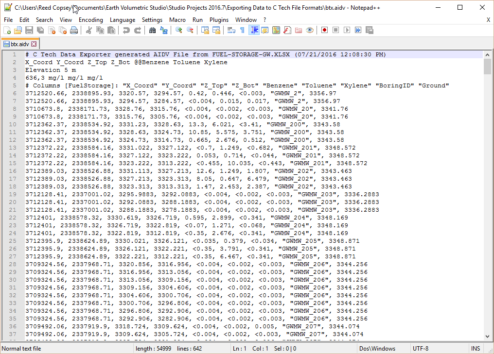
Our last two tasks will be to take a look at the file in a text editor and confirm that it works in Earth Volumetric Studio.

Although Windows comes with Notepad, it is really a very poor text editor since it lacks line numbers, column numbers, and the ability to handle large files. There are many freeware text editors, but the one we like is Notepad++.

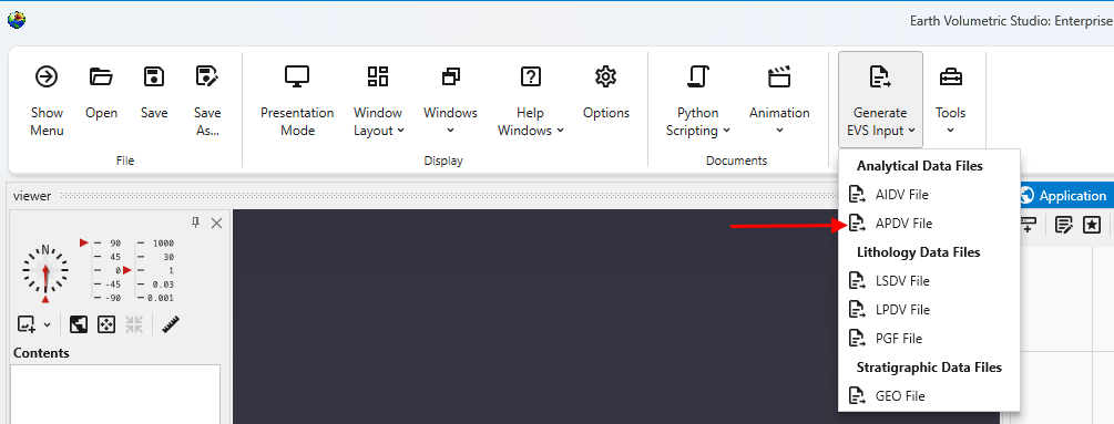
Begin by selecting the “Generate EVS Input” button in the Main Toolbar, and select APDV File.

Note: this topic builds upon Creating AIDV Files and assumes that you have completed that topic.

Let’s browse to the folder shown and select the file Railyard-soil.xlsx

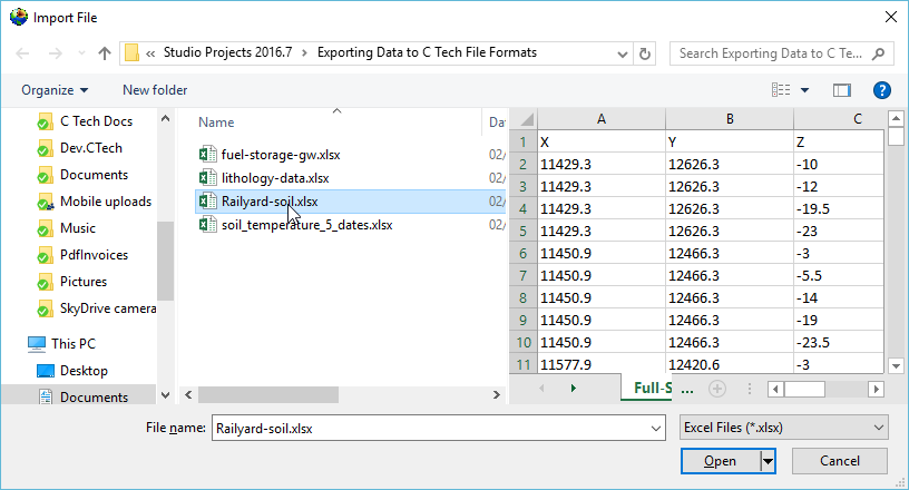
This file has three sheets and for this example, we’ll choose the second one. This particular sheet has Z coordinates represented as both true Elevation and Depth below ground surface. Both are commonly used and it is not uncommon to see both in a database as a convenience for people working with the data. Our exporter can use either one and there is no technical advantage of one over the other. However, the data file created will retain the Z coordinate option selected.

Since we used True Elevations for AIDV files, let’s work with Depths this time. The correct settings are:

Please note that Top, which is our Ground Surface must be in true elevation since it is the reference surface used to define depths. Depths are always positive numbers with greater depth corresponding to lower elevations.

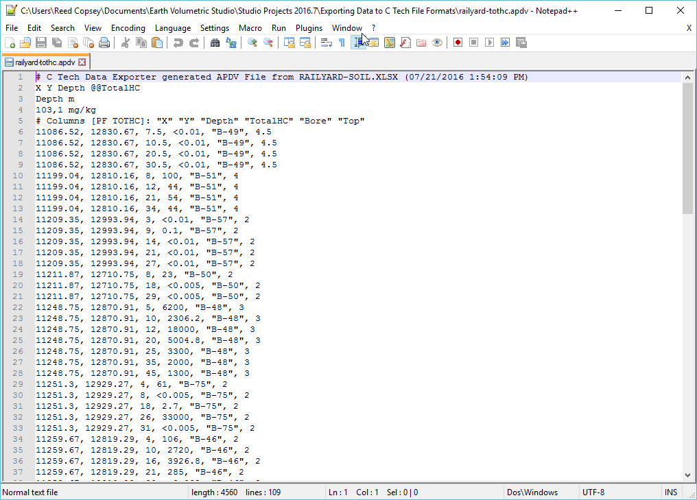
With all of our settings correct as shown above, all we need to do is click the Generate APDV File button, and let’s call the file railyard-tothc.apdv.

In notepad++ our file looks like:

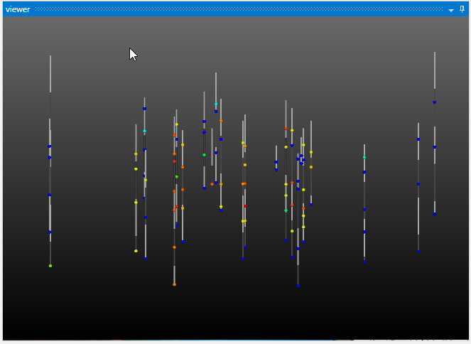
and if we look at this file in Studio with Z-Scale of 5 it is:

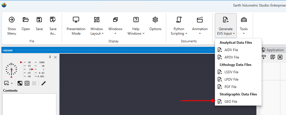
Begin by selecting the “Generate EVS Input” button in the Main Toolbar, and select GEO File.

Let’s browse to the folder shown and select the file fuel-storage-gw.xlsx since we mentioned that this file had three surface which we can use for stratigraphic geology. In this case the three surfaces define just two layer which correspond to the vadose and saturated regions, however, that is an important minimal geology file for working with groundwater data.

If we select the only table, choose the correct settings and scroll to the far right we can see the fields that represent our bottom two surfaces:

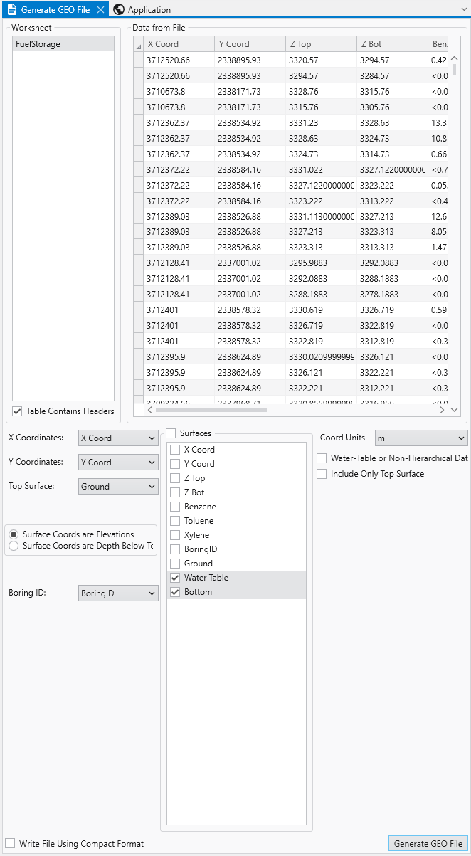
Based on the values for both surfaces, it is clear they are Elevations and not Depths. For the Surfaces selectors, we don’t choose Ground because it is already selected as the Top Surface. This file will have three surfaces defining two layers.

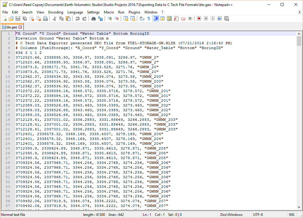
With all of our settings correct as shown above, all we need to do is click the Generate AIDV File button, and let’s call the file btx.geo.

Since geo files are rather boring in post_samples, let’s do something a bit more interesting with this data.

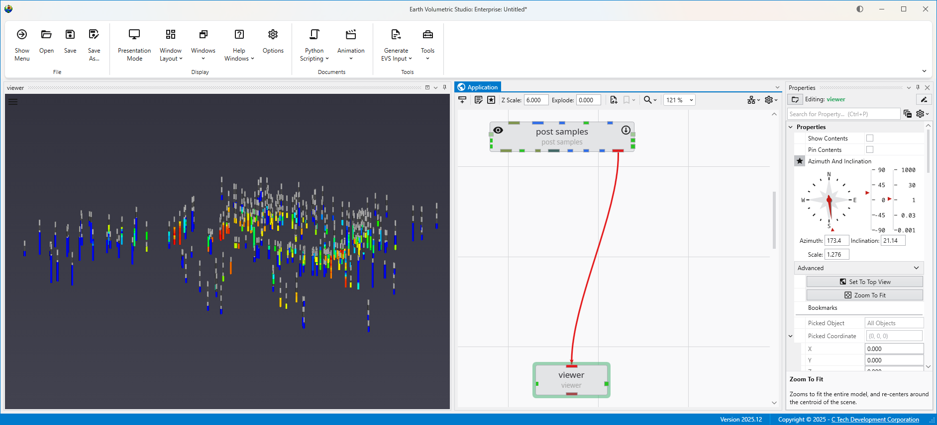
Below is our application and its output. We cheated a bit and I want to explain where and why.

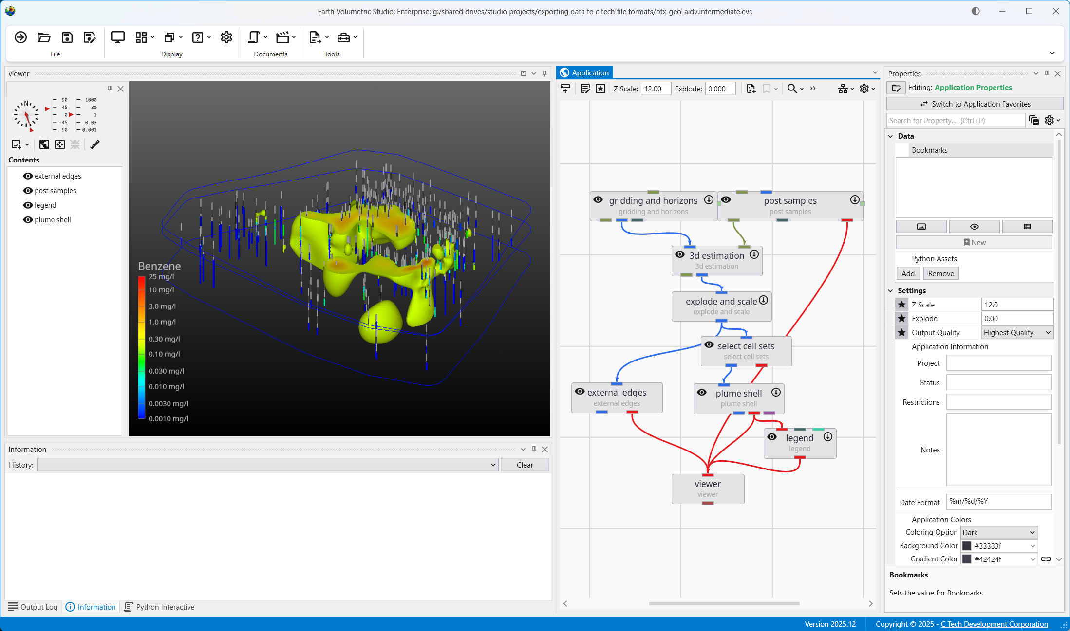
We’ve kriged groundwater data into both layers of our model. However it doesn’t make sense to ever display or do any volumetric analysis of groundwater data in the vadose zone. We could have used the subset horizons module to get only the single bottom layer corresponding to the saturated zone (aquifer) but if we did that, we wouldn’t have both stratigraphic layers which we are displaying with the external_edges module and could display with a variety of other techniques. In that case we would need to create a parallel path in our application where we would use horizons to 3d to create either the top layer only or both layers in order to display the geology separate from the groundwater chemistry.

So we cheated and kriged into both layers, but we used the select cell sets module to turn off the upper layer before we display the plume with plume_shell. If we wanted to do volumetrics, we would be sure to only do so for the bottom layer. Other than a few seconds used to krige into the vadose layer we’ve managed to get by with a simpler application.

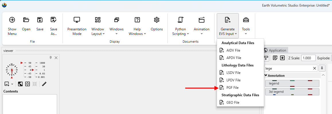
Begin by selecting the “Generate EVS Input” button in the Main Toolbar, and select PGF File.

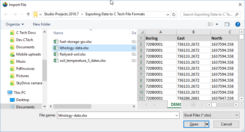
We’ll choose lithology-data.xlsx and its only table, DEMO.

When you look at the table, it is clear that we have a Start and End (Top and Bottom), which means that we need to select the “Rows Are Intervals” toggle in the upper left. This toggle allows us to select separate X-Y-Z coordinates for the Start and End to handle non-vertical borings, but if the borings are vertical, both X and Y columns can be the same.

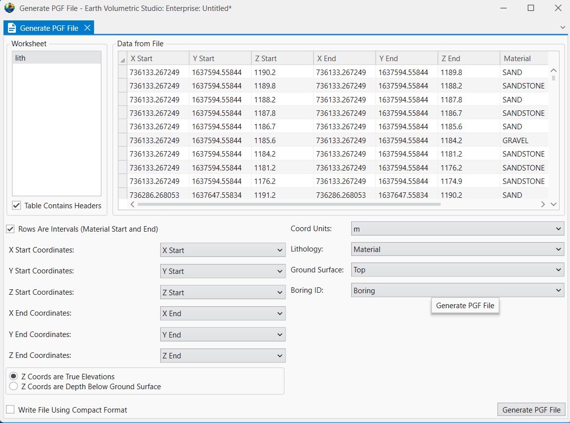
This is another table where we could work in Depths or Elevations. However for a PGF file, the file itself is always in Elevation, so if you choose depth, it just does the conversion before creating the file. We’ll just use the elevation fields directly. However, always make sure you’ve selected the right ones and be consistent.

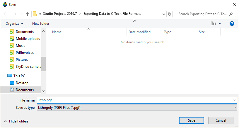
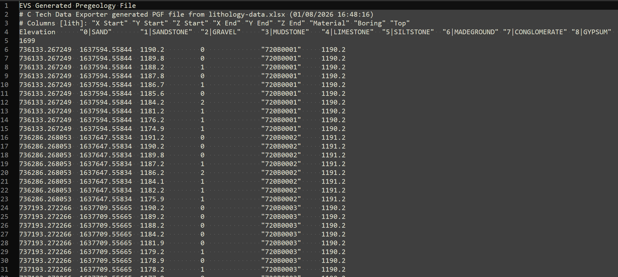
With all of our settings correct as shown above, all we need to do is click the Generate PGF File button, and let’s call the file litho.pgf.

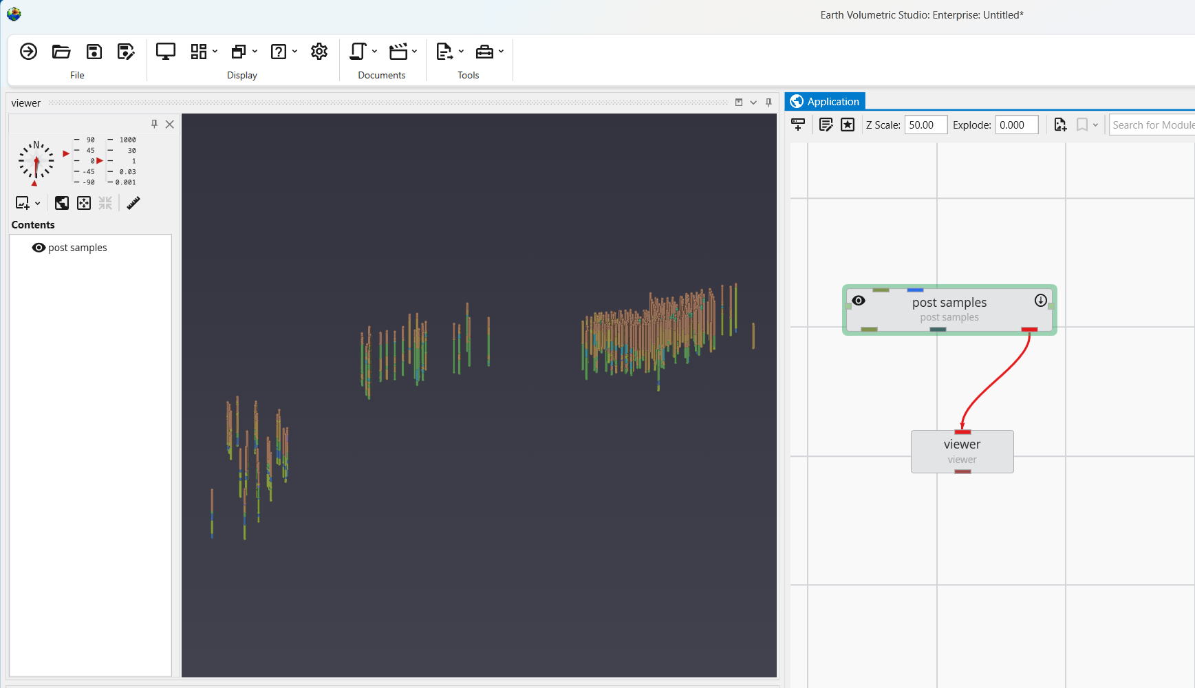
Below is the file in Notepad++

We can now load this file in post samples, where we can see that this dataset spans a very large set with borings in three distinct groupings. We need a Z-Scale of 50 to be able to see the borings well.